2026-07-21

I spent some time exploring the parameter space for the example given in 2026-07-09. More specifically, I modified the weights of triangles as follows:

$$v_i=\{\begin{array}{ll}{\theta }_1& \text{ if yi is not a Mobius triangle}\\ {\theta }_2& \text{ if yi is a Mobius triangle.}\end{array}$$

I then did an exhaustive computation of $({\theta }_1,{\theta }_2)\in [0.1,3]\times [0.1,3]$ with a step size of $\Delta {\theta }_i=0.01$. For each set of weights, I solved the flat norm LP and stored the objective value $z^{\ast }$, and whether ${\mathbf{y}}^{\ast }$ is integral. In other words, I looked at the following map:

$$f({\theta }_1,{\theta }_2)=\{\begin{array}{ll}(z^{\ast },1)& \text{if }{\mathbf{y}}^{\ast }\in {\mathbb{Z}}^n\\ (z^{\ast },0)& \text{if }{\mathbf{y}}^{\ast }\notin {\mathbb{Z}}^n.\end{array}$$

I then plotted this map using a contour plot:

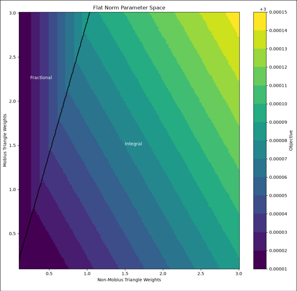
We find the following interesting facts:

• Every fractional solution $(z^{\ast },{\mathbf{x}}^{\ast },{\mathbf{y}}^{\ast })$ has a corresponding integral solution with the same objective $z^{\ast }$.
• For each objective value $z^{\ast }$, its corresponding parameter space is divided into two parts: fractional vertices and integral vertices.

My idea is as follows:

1. Compute the flat norm LP
2. If the solution is fractional, tweak the weights so that we get an equivalent integral solution.

Parameter Space and It’s Tangent Space

This strategy requires us to have a strong understanding of the parameter space. That is, fix $K$ and $c$ and look at the space $\theta =(\mathbf{w},\lambda \mathbf{v})$. Assume that the LP gave $z=3.00009$ as in our example. For any vertex of the LP $u=(\mathbf{x},\mathbf{y})$, consider $g(u)=({\mathbf{x}}^{+}+{\mathbf{x}}^{-},{\mathbf{y}}^{+}+{\mathbf{y}}^{-})$. Then our objective is given by

$$z(\theta ,u)=⟨\theta ,g(u)⟩=\sum _{i=1}^N{\theta }_{i}g(u{)}_i.$$

We want to look at the following hypersurface in ${\mathbb{R}}_{\ge 0}^{2N-1}$ where $N=m+n$:

$$\begin{array}{rl}{\mathcal{S}}_{z^{\ast }}& =\{\theta \ge 0,u\ge 0:z(\theta ,u)=z^{\ast }\}\\ & =\{\theta \ge 0,u\ge 0:\sum _{i=1}^N{\theta }_i(g(u){)}_i=z^{\ast }\}.\end{array}$$

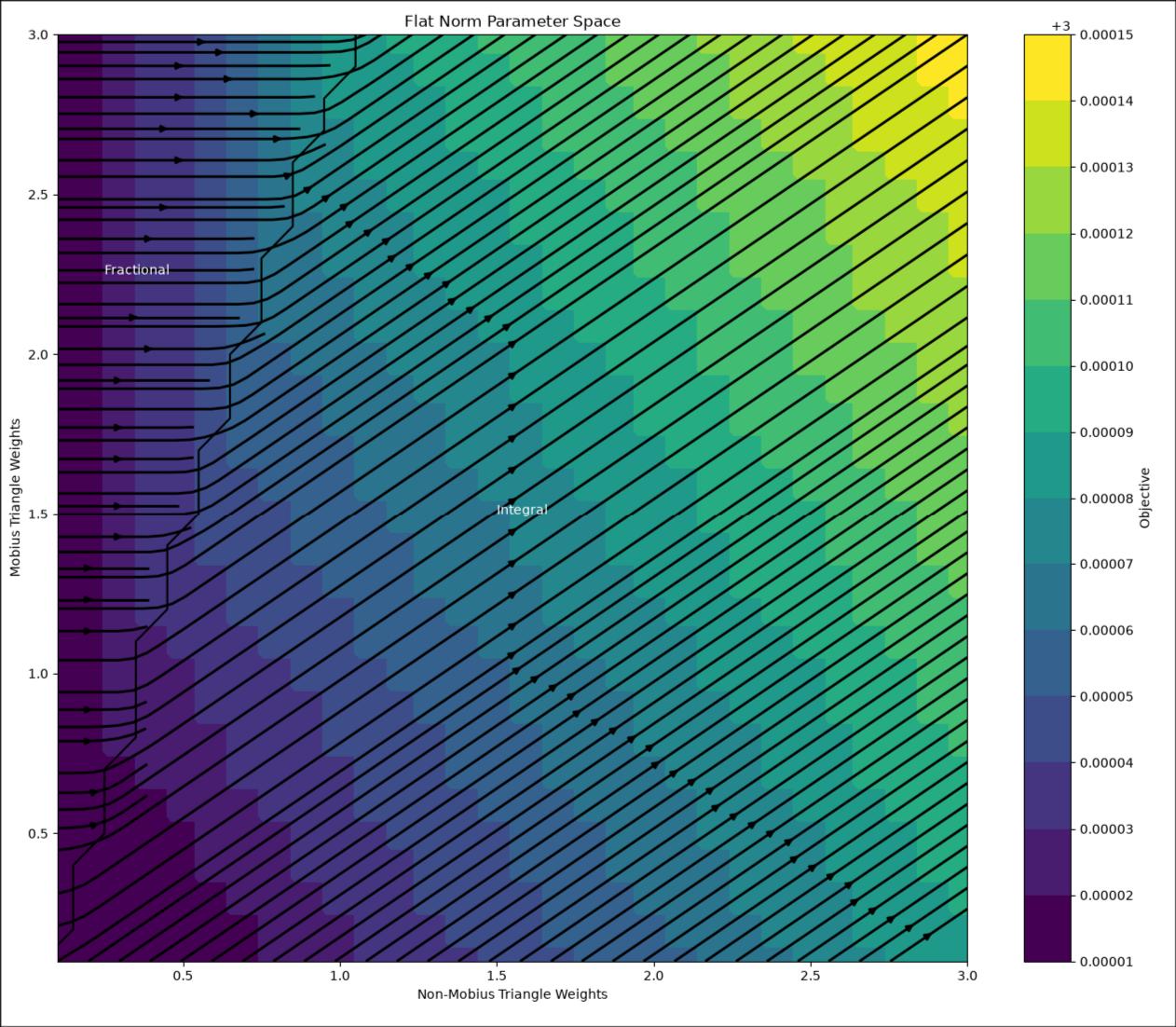
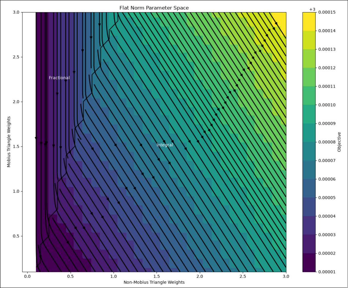
Notice that the map $z:{\mathbb{R}}^{2N}\to \mathbb{R}$ is smooth and ${\nabla }_{\theta }z=g(u)$ on $\mathcal{S}$. Experimentation suggests that ${\nabla }_{\theta }z$ is orthogonal to the direction we need to travel, i.e., we need to nudge $\theta$ tangent to ${\nabla }_{\theta }z$:

Gradient ${\nabla }_{\theta }z$ projected to $(w1,w2)$ space:

Tangent $(v,-u)$ of the gradient:

In our higher dimension, we want to look at the tangent space:

$$T_{\theta }=\{v\in {\mathbb{R}}^N:g(u{)}^{\top }v=0\}.$$

However, there are a ton of options to choose from! In the 2D picture we took

$$v=e_1-\frac{e_1^{\top }g(u)}{g(u{)}^{\top }g(u)}g(u)\in T_{\theta }.$$

If we want an orthonormal basis for $T_{\theta }$, we could use a Householder reflection and compute the QR decomposition of $g(u)$ (viewed as a $N\times 1$ matrix). Set $\hat{g}=g(u)/\Vert g(u)\Vert$ and $\alpha =\text{sgn}(g_1)$. Then the QR decomposition is given by

$$Q=I-2\mathbf{u}{\mathbf{u}}^{\top }\text{ where }\mathbf{u}=\frac{\hat{g}-\alpha e_1}{\Vert \hat{g}-\alpha e_1\Vert }.$$

Then for any $\gamma \in {\mathbb{R}}^{N-1}$,

$$g(u{)}^{\top }\left(\sum _{i=1}^{N-1}{\gamma }_i{Q}_{i+1}\right)=0,$$

i.e., the columns $2,\dots ,N$ of $Q$ form a basis for $T_{\theta }$.

Proof. Denote by $G=\Vert \hat{g}-\alpha e_1\Vert$. Notice that for $j\ge 2$,

$$u_j=\frac{(\hat{g}-\alpha e_1{)}_j}{G}=\frac{{\hat{g}}_j-\alpha (e_1{)}_j}{G}=\frac{{\hat{g}}_j}{G}$$

and

$$G^2=(\hat{g}-\alpha e_1{)}^{\top }(\hat{g}-\alpha e_1)={\hat{g}}^{\top }\hat{g}-\alpha {\hat{g}}^{\top }{e}_1-\alpha e_1^{\top }\hat{g}+{\alpha }^2{e}_1^{\top }{e}_1=1-2\alpha {\hat{g}}_1+{\alpha }^2=2(1-\alpha {\hat{g}}_1)$$

as ${\alpha }^2=1$. Thus,

$$\begin{array}{rl}{\hat{g}}^{\top }(Q{e}_j)& ={\hat{g}}^{\top }(e_j-2\mathbf{u}{\mathbf{u}}^{\top }{e}_j)\\ & ={\hat{g}}^{\top }\left[e_j-2({\mathbf{u}}^{\top }{e}_j)\mathbf{u}\right]\\ & ={\hat{g}}^{\top }\left[e_j-2u_j\mathbf{u}\right]\\ & ={\hat{g}}_j-2u_j{\hat{g}}^{\top }\mathbf{u}\\ & ={\hat{g}}_j-2\left(\frac{{\hat{g}}_j}{G}\right)\left(\frac{{\hat{g}}^{\top }(\hat{g}-\alpha e_1)}{G}\right)\\ & ={\hat{g}}_j-2\left(\frac{{\hat{g}}_j}{G}\right)\left(\frac{{\hat{g}}^{\top }\hat{g}-\alpha {\hat{g}}^{\top }{e}_1)}{G}\right)\\ & ={\hat{g}}_j-2\left(\frac{{\hat{g}}_j}{G}\right)\left(\frac{1-\alpha {\hat{g}}_1}{G}\right)\\ & ={\hat{g}}_j-\frac{2{\hat{g}}_j(1-\alpha {\hat{g}}_1)}{G^2}\\ & ={\hat{g}}_j-\frac{2{\hat{g}}_j(1-\alpha {\hat{g}}_1)}{2(1-\alpha {\hat{g}}_1)}\\ & =0.\end{array}$$

Orthonormal is left as an exercise. $\square$

While we can compute an orthonormal basis for $T_{\theta }$, it is unclear which tangent we should take. However, if we could find the “best” one, then we would have an algorithm to find an integral solution given a fractional.

The Algorithm

Denote the tangent to ${\nabla }_{\theta }z=g(u)$ by $\tau (u)$. One approach to this is as follows:

1. Set ${\theta }_0$ by the given parameters.
2. Solve the flat norm LP to find $u_0$, record the objective value $z^{\ast }$.
3. At step $k$, do the following:
   1. If $u_k\in {\mathbb{Z}}^N$, stop.
   2. Otherwise, set ${\theta }_{k+1}={\theta }_k+{\rho }_k\tau (u_k)$
   3. Find $u_{k+1}$ such that $({\theta }_{k+1},u_{k+1})\in {\mathcal{S}}_{z^{\ast }}$.

The difficult step is projecting back into ${\mathcal{S}}_{z^{\ast }}$. Let $u_{k+1}=\mu u_k$. Notice that

$$\begin{array}{rl}{z}^{\ast }& =z({\theta }_{k+1},u_{k+1})\\ & =⟨{\theta }_{k+1},\mu u_k⟩\\ & =\mu ⟨{\theta }_{k+1},u_k⟩\end{array}$$

implies that

$$\mu =\frac{z^{\ast }}{⟨{\theta }_{k+1},u_k⟩}.$$

So, we get back to ${\mathcal{S}}_{\ast }$ by setting

$$u_{k+1}=\frac{z^{\ast }}{⟨{\theta }_{k+1},u_k⟩}{u}_k.$$

However, this doesn’t respect the homology constraints. Notice that

$$\begin{array}{rl}\mu ({\mathbf{x}}^{+}-{\mathbf{x}}^{-})-\mu B({\mathbf{y}}^{+}-{\mathbf{y}}^{-})& =\mu \mathbf{c}\ne \mathbf{c}.\end{array}$$

Notice that if we set ${\mathbf{u}}_{k+1}=(\mathbf{x}+ϵ,\mathbf{y}+\delta )$, then

$$⟨\theta ,(\mathbf{x}+ϵ,\mathbf{y}+\delta )⟩=⟨\theta ,\mathbf{u}⟩+⟨\theta ,(ϵ,\delta )⟩=z^{\ast }+⟨\theta ,(ϵ,\delta )⟩.$$

What we need to do, is solve the following LP:

$$\begin{array}{rlr}& \text{minimize}& \Vert ϵ\Vert +\Vert \delta \Vert \\ & \text{subject to}& ⟨{\theta }_{k+1},(ϵ,\delta )⟩=0\\ & & (\mathbf{x}+ϵ)-B(\mathbf{y}+\delta )=\mathbf{c}\\ & & ϵ,\delta \in {\mathbb{R}}^N.\end{array}$$

Call this problem $\mathcal{P}2$ and the flat norm $\mathcal{P}1$. Then our algorithm is as follows:

1. Set ${\theta }_0$ by the given parameters.
2. Solve $\mathcal{P}1$ to find $u_0$, record the objective value $z^{\ast }$.
3. At step $k$, do the following:
   1. If $u_k\in {\mathbb{Z}}^N$, stop.
   2. Otherwise, set ${\theta }_{k+1}={\theta }_k+{\rho }_k\tau (u_k)$
   3. Find $u_{k+1}$ by solving $\mathcal{P}2$.
4. Compute $z(\theta ,u⟩$ with the original parameters ${\theta }_0$.

However, I don’t know if this will converge in a linear number of steps. We would likely need a good step size to ensure it doesn’t overshoot. It would also be great if we could quickly solve $\mathcal{P}2$.

---

Update 7/24/26: I implemented this approach with the exception that I find $u_{k+1}$ by solving the flat norm problem with the new weights instead of solving $\mathcal{P}2$. The algorithm converged to an integral solution. Moreover, the solution was the exact integral solution! For a step size, I used

$${\rho }_k=\frac{1}{(k+1)\Vert g(u){\Vert }^2}.$$

Initial Solution:
  z = 3.00004
  x = 0.5*[3,4] + 0.5*[0,1] + 0.5*[1,2] + 0.5*[4,5] + 0.5*[2,3] + -0.5*[0,5]
  y = 0.5*[3,4,6] + 1*[0,4,6] + -0.5*[0,3,6] + -0.5*[1,4,6] + -0.5*[0,1,6] + -1*[4,6,7] + 0.5*[1,4,7] + -1*[2,4,7] + -0.5*[1,2,7] + 0.5*[4,5,7] + -0.5*[5,7,8] + -0.5*[2,7,8] + -0.5*[2,3,8] + -0.5*[0,5,8] + -0.5*[0,3,8]
Iteration 1:
  grad=(3, 9); step=0.000123457; w=(0.6, 1.46667)
  z = 3.00005
  x = 1*[6,7] + 1*[7,8] + -1*[6,8]
  y = -1*[0,1,4] + -1*[1,2,4] + -1*[2,3,8] + -1*[0,3,8] + -1*[3,6,8]
Converged!

Solution:
  z = 3.00004
  x = 1*[6,7] + 1*[7,8] + -1*[6,8]
  y = -1*[0,1,4] + -1*[1,2,4] + -1*[2,3,8] + -1*[0,3,8] + -1*[3,6,8]

Solution verified by Gurobi (with integer constraints):

$$\begin{array}{rl}{z}^{\ast }& =3.00004\\ x& =[6,7]+[7,8]-[6,8]\\ y& =-[0,1,4]+[1,4,7]-[2,4,7]-[1,2,7]-[2,3,8]-[0,3,8]-[3,6,8]\end{array}$$

ampl: model flatnorm.mod;
ampl: option solver gurobi;
ampl: solve;
Gurobi 13.0.2: optimal solution; objective 3.000045
42 simplex iterations
1 branching node
ampl: display Obj;
Obj = 3.00004

ampl: display xp;
xp [*] :=
 0 0    3 0    6 0    9 1   12 0   15 0   18 1   21 0   24 0
 1 0    4 0    7 0   10 0   13 0   16 0   19 0   22 0   25 0
 2 0    5 0    8 0   11 0   14 0   17 0   20 0   23 0   26 0
;

ampl: display xm;
xm [*] :=
 0 0    3 0    6 0    9 0   12 0   15 0   18 0   21 0   24 0
 1 0    4 0    7 0   10 0   13 0   16 0   19 0   22 0   25 0
 2 0    5 0    8 0   11 0   14 0   17 0   20 0   23 0   26 1
;

ampl: display yp;
yp [*] :=
 0 0    3 0    6 0    9 1   12 0   15 0   18 0   21 0   24 0
 1 0    4 0    7 0   10 0   13 0   16 0   19 0   22 0   25 0
 2 0    5 0    8 0   11 0   14 0   17 0   20 0   23 0   26 0
;

ampl: display ym;
ym [*] :=
 0 0    3 0    6 1    9 0   12 0   15 0   18 0   21 0   24 0
 1 0    4 0    7 0   10 1   13 0   16 0   19 0   22 0   25 1
 2 0    5 0    8 0   11 1   14 0   17 0   20 1   23 1   26 0
;