Circuit Simulation

A circuit can be viewed as having $n$ nodes, a ground node, and $b$ branches; where a node is a junction where current can split or combine, and a branch represents a path in the circuit containing one or more components in series connecting two nodes. This results in a directed graph $G=(V,E)$ where $V$ corresponds to nodes and $E$ corresponds to branches. The graph $G$ can be encoded as an $(n+1)\times b$ incidence matrix $A_{inc}$ by denoting $+1$ for the source of a directed edge, and $-1$ for the destination as shown below:

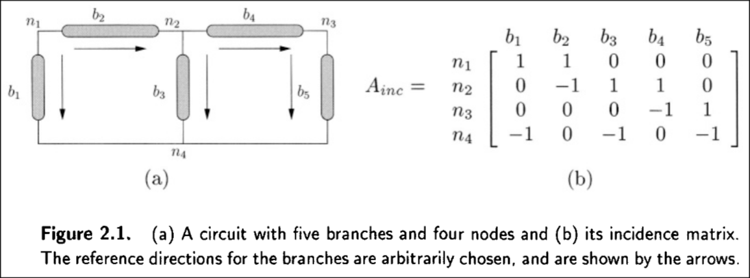
Let ${\mathbf{I}}_{\mathbf{b}}\in {\mathbb{R}}^b$ denote the vector of signed branch currents, ${\mathbf{V}}_{\mathbf{b}}\in {\mathbb{R}}^b$ denote the vector of branch voltages, and ${\mathbf{V}}_{\mathbf{n}}\in {\mathbb{R}}^{n+1}$ denote the vector of node voltages. Then it follows from Kirchoff’s circuit laws that

$$A{\mathbf{I}}_{\mathbf{b}}=0\text{ and }{A}^{\top }{\mathbf{V}}_{\mathbf{n}}={\mathbf{V}}_{\mathbf{b}}.$$

That is, the algebraic sum of the current entering/leaving node $i$ is zero and the voltage across a branch is given by the difference between the voltages at either end.

Given the above, we describe the relation between ${\mathbf{V}}_{\mathbf{b}}$ and ${\mathbf{I}}_{\mathbf{b}}$ through device equations. These equations could be linear, non-linear, or differential equations. For now we focus on two types:

• Type 1 devices are defined by the equation ${\mathbf{I}}_b=Y{\mathbf{V}}_{\mathbf{b}}+\mathbf{s}$, where $Y$ is a $b_1\times b_1$ matrix, $\mathbf{s}$ is a $b_1\times 1$ vector and $b_1$ is the number of type 1 devices. Examples include conductances, constant current sources, and voltage-controlled current sources.
• Type 2 devices are defined by the equation $Z{\mathbf{I}}_{\mathbf{b}}+G{\mathbf{V}}_{\mathbf{b}}=\mathbf{t}$, where $Z$ and $G$ are $b_2\times b_2$ matrices and $\mathbf{t}$ is a $b_2\times 1$ vector. Examples include constant voltage sources and current-controlled current/voltage sources.

We rearrange our incidence matrix such that $A_{inc}=\left[\begin{array}{cc}{A}_1& A_2\end{array}\right]$ so that $A_1$ ($A_2$) is the submatrix corresponding to Type 1 (Type 2) devices. Then we can describe the circuit by the following system of equations:

$$\begin{array}{rlrl}\text{KCL}:& & A_1{\mathbf{I}}_{{\mathbf{b}}_1}+A_2{\mathbf{I}}_{{\mathbf{b}}_2}& =0\\ \text{KVL}:& & {\mathbf{V}}_{b_1}& =A_1^{\top }{\mathbf{V}}_{\mathbf{n}}\\ & & {\mathbf{V}}_{b_2}& =A_2^{\top }{\mathbf{V}}_{\mathbf{n}}\\ \text{Device Equations:}& & {\mathbf{I}}_{{\mathbf{b}}_1}& =Y{\mathbf{V}}_{{\mathbf{b}}_1}+\mathbf{s}\\ & & Z{\mathbf{I}}_{{\mathbf{b}}_2}+G{\mathbf{V}}_{b2}& =\mathbf{t}\end{array}$$

Combining equations together gives us the modified nodal formulation (MNA):

$$\left[\begin{array}{cc}{A}_{1}Y{A}_1^{\top }& A_2\\ G{A}_2^{\top }& Z\end{array}\right]\left[\begin{array}{c}{\mathbf{V}}_{\mathbf{n}}\\ {\mathbf{I}}_{{\mathbf{b}}_2}\end{array}\right]=\left[\begin{array}{c}-A_1\mathbf{s}\\ \mathbf{t}\end{array}\right].$$

Notice that the MNA equation only has variables for the node voltages, ${\mathbf{V}}_{\mathbf{n}}$, and the currents through the Type 2 elements, ${\mathbf{I}}_{{\mathbf{b}}_2}$. If there are no Type 2 elements, then this simplifies to $Y{A}_1^{\top }{\mathbf{V}}_{\mathbf{n}}=-\mathbf{s}$ and is called the nodal formulation.

Non-linear device equations are often captured by a first-order Taylor series expansion. For instance a device of the form $f(x_1,x_2,\dots ,x_n)=0$ can be approximated by taking the first-order Taylor series about the point ${\mathbf{x}}_k$:

$$f(x_1^k,x_2^k,\dots ,x_n^k)+\sum _{i=1}^n\left(\frac{\partial f(x_1,x_2,\dots ,x_n)}{\partial x_i}{|}_{{\mathbf{x}}_{\mathbf{k}}}(x_i-x_i^k)\right)=0.$$

The expansion point ${\mathbf{x}}_k$ is updated identical to Newton’s method. A more general framework combines all devices, linear and nonlinear, using the Jacobian:

$$J({\mathbf{x}}_k)\mathbf{x}=-\mathbf{f}({\mathbf{x}}_{\mathbf{k}})+J({\mathbf{x}}_{\mathbf{k}}){\mathbf{x}}_k.$$

Devices can also be described by differential equations; in such a case, one may use methods such as Euler’s method to numerically approximate their solution. This all cumulates into the following simulation pipeline:

1. At each iteration $k$:
   1. For the current time step $t_k$, convert the differential equations into nonlinear and linear equations
   2. Linearize nonlinear equations to obtain a system of linear equations
   3. Solve the system of linear equations
   4. If we have simulated the desired time period, stop. Otherwise, increment the current time step $t_{k+1}=t_k+\Delta t$ and continue to iteration $k+1$.