Persistent Homology

Consider a filtration on a simplicial complex $K$:

$$\varnothing =K^0\subset K^1\subset \cdots \subset K^m=K.$$

Then we can consider the homology group of each subcomplex $K^{\ell }$ in the filtration:

$$H_p(K^{\ell })=Z_p(K^{\ell })/B_p(K^{\ell }),\ell =0,1,\dots ,m$$

As a result we also get the Betti numbers

$${\beta }_p(K^{\ell })=\text{rank}{H}_p(K^{\ell }).$$

Notice that the inclusion map ${\iota }^{i,j}:K^i\hookrightarrow K^j$, $i\le j$, induces the homomorphism $f_p^{i,j}:H_p(K^i)\to H_p(K^j)$.

Persistent Homology Group

The p-persistent k-th Homology group of $K^{\ell }$ is given by

$$H_k^{\ell ,\ell +p}=\text{Im}{f}_k^{\ell ,\ell +p}=Z_k(K^{\ell })/(B_k(K^{\ell +p})\cap Z_k(K^{\ell }))$$

and ${\beta }_k^{\ell ,\ell +p}=\text{rank}{H}_k^{\ell ,\ell +p}$ is the p-persistent k-th Betti number of $K^{\ell }$.

In other words, $H_k^{\ell ,p}$ are all $k$-cycles in $K^{\ell }$ that are not $k$-boundaries in $K^{\ell },\dots ,K^{\ell +p}$ (note $B_k(K^{\ell })\subseteq B_k(K^{\ell +1})$).

We can gather information on the complex by tracking ${\beta }_p^{\ell }={\beta }_p(K^{\ell })$ for fixed $p$ and varying $\ell$. For example,

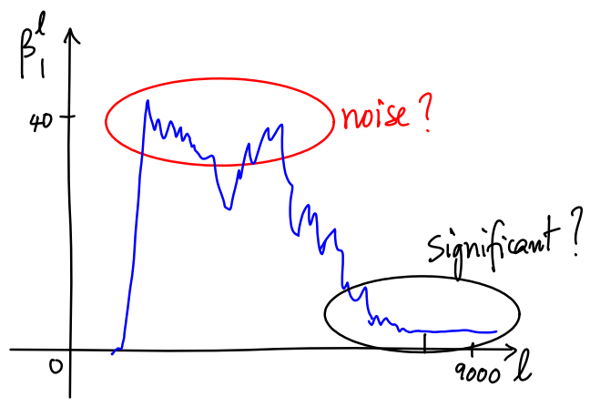
in the plot above we see early on there are a lot of holes (recall ${\beta }_1$ represents the number of holes) in the complex that get “filled” later on. However, initially there is a lot of noise. We expect any significant feature of the space to have a long “lifetime”. In otherwords, we want to look for cycles in $K^{\ell }$ that are not boundaries until $K^{\ell +p}$ for some time step $p$.

Assume that the non-boundary $k$-cycle $z$ is created at time $i$ with the inclusion of simplex ${\sigma }^i$. Then $[z]\in H_k^i$. Assume that at time $j$, $z^{\prime }\in [z]$ becomes a $k$-boundary with the inclusion of simplex ${\sigma }^j$, that is, the hole captured by $[z]$ is closed by ${\sigma }^j$. Then $z^{\prime }\in B_k(K^j)$ and the class $[z]$ is merged with an older class of cycles.

Persistence and Lifetime

Let $z$ be a non-boundary $k$-cycle. If $[z]$ is created by ${\sigma }^i$ at time $i$, then ${\sigma }^i$ is the creator of $[z]$. If $[z]$ is destroyed by ${\sigma }^j$ at time $j$, i.e., $[z]$ merges with an older class, then ${\sigma }^j$ is the destroyer of $[z]$. We say $[i,j)$ is the lifetime of $[z]$ and that the persistence of $[z]$ is $j-i-1$.

Some classes may not have a destroyer. In such a case, its persistence is $\infty$.

Fundamental Lemma of Persistent Homology

Our goal is count the number of classes that are born in $K^i$ and die in $K^j$. Notice that ${\beta }_k^{i,j}$ represents the number of classes in $H_p(K^i)$ that are still alive in $H_p(K^j)$. As result, the number of classes that are alive in $H_p(K^i)$ but die entering $H_p(K^j)$ is given by

$${\beta }_p^{i,j-1}-{\beta }_p^{i,j}.$$

Similarly, the number of classes alive in $K^{i-1}4thatdiein$K^j$ is given by

$${\beta }_p^{i-1,j-1}-{\beta }_p^{i-1,j}.$$

Therefore,

$${\mu }_p^{i,j}=({\beta }_p^{i,j-1}-{\beta }_p^{i,j})-({\beta }_p^{i-1,j-1}-{\beta }_p^{i-1,j})$$

is the number of p-dimensional classes that are born at $K^i$ and die entering $K^j$.

Fundamental Lemma of Persistent Homology

$${\beta }_p^{k,\ell }=\sum _{i\le k}\sum _{j>\ell }{\mu }_p^{i,\ell }\text{ for }k\le \ell$$

Persistence Diagrams

We pair a creator ${\sigma }^i$ with a destroyer ${\sigma }^j$ to capture a specific $p$-dimensional class. The persistence diagram is formed by taking all such pairs $({\sigma }^i,{\sigma }^j)$ and plotting their indices on the index-index plane.

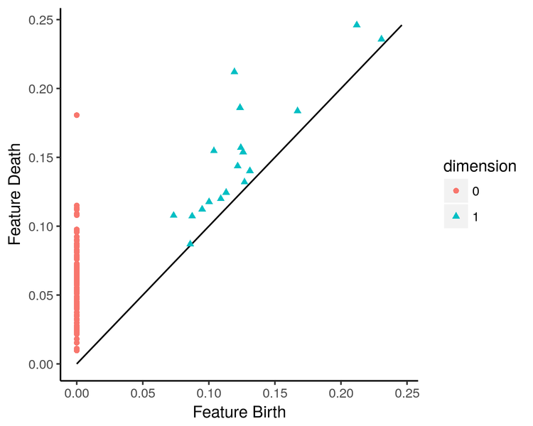
Under the assumption that we have a monotonic filtration (all proper faces already exist when $\sigma$ enters), then we get that $i<j$ for all pairs.

So we say the persistence is the vertical distance from the $i=j$ line. We can use persistence diagrams to calculate the persistent Betti numbrs:

${\beta }_p^{k,\ell }$ is given by the number points (with multiplicities) in the upper left quadrant with corner $(k,\ell )$.

We can compute the pairings using the “combined boundary matrix”.

Combined Boundary Matrix

Let $\varnothing =K^0\subset K^1\subset \cdots \subset K^m$ be a monotonic filtration. We construct the $m\times m$ matrix $[\partial ]$ by

$$[\partial {]}_{ij}=\{\begin{array}{ll}1& \text{if σi≺σj and dimσi=dimσj−1}\\ 0& \text{otherwise}.\end{array}$$

The matrix captures the filtration in the order of rows and columns. We will use replacement column operations over ${\mathbb{Z}}_2$ to “reduce” the matrix.

low, reduced

Let $low(j)$ be the row index of the lowest 1 in column j. We call a matrix $R$ reduced if $low(j)\ne low(j^{\prime })$ whenever $j\ne j^{\prime }$ for non-zero columns of $R$.

The reduction algorithm moves through columns left to right, adding any columns $j^{\prime }$ to the left of $j$ where $low(j)=low(j^{\prime })$.

void REDUCE
    R = combined boundary matrix
    for j=1 to m
        while there is some j'<j such that low(j)=low(j')
            add column j' to column j
        end
    end
end

This algorithm is quite slow with run time of $O(m^3)$.

After the reduction is finished, the pairings are given by $(j,low(j))$ for non-zero columns $j$.