Local Descent

When optimizing multivariate functions a common approach is to make use of local models and incrementally improve a point. We can do this by at each iteration choosing a direction of descent and stepping in the descent direction with an appropriate step size. The local model is often built via a Taylor approximation. The general flow of descent direction methods is as follows:

1. Check if ${\text{x}}^{(k)}$ satisfies the termination condition, if so, terminate.
2. Calculate the descent direction ${\text{d}}^{(k)}$.
3. Determine the step size (aka as learning rate) ${\alpha }^{(k)}$.
4. Compute the next design point ${\text{x}}^{(k+1)}={\text{x}}^{(k)}+{\alpha }^{(k)}{\text{d}}^{(k)}$.

Gradient Descent

A natural choice for the descent direction $\text{d}$ would be the direction of steepest descent. Luckily this is also equal to the opposite direction of the gradient $\nabla f$. We often normalize,

$${\text{d}}^{(k)}=-\frac{\nabla f({\text{x}}^{(k)})}{\Vert \nabla f({\text{x}}^{(k)})\Vert }.$$

Resulting in the following simple algorithm:

x = x0
for k in range(k_max):
	d = grad_f(x)
	x = x - alpha * d / norm(d)

Line Search

For step 3 of the method, we need to determine our step size. One approach is known as line search which chooses the step factor that minimizes some objective function:

$$\underset{x}{\mathrm{minimize}}f(\text{x}+\alpha \text{d})$$

This is a univariate optimization problem and can be solved using Bracketing. However, this process can be quite slow and finding the optimal step size $\alpha$ at a high degree of precision is often unnecessary. Some algorithms simply use a fixed step factor. Another common method is to use a decaying step factor

$${\alpha }^{(k)}={\alpha }^{(1)}{\gamma }^{k-1}$$

where $\gamma \in (0,1]$. A decaying step factor is a popular choice when the objective function is noisy.

In order for our descent method to function properly, our step size needs to be suitable, i.e., result in a decrease in the objective function. The condition for sufficient decrease, sometimes referred to as Armijo condition, is that

$$f({\text{x}}^{(k+1)})\le f({\text{x}}^{(k)})+\beta \alpha {\nabla }_{{\text{d}}^{(k)}}f({\text{x}}^{(k)})$$

with $\beta \in [0,1]$ often set to $\beta =1\times 10^{-4}$. This condition is visualized in the figure below.

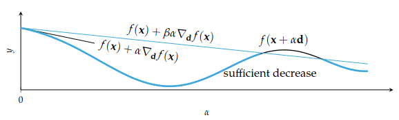
As long as $\text{d}$ is a valid descent direction, a sufficiently small step size exists. The algorithm backtracking line search starts with a large step size and decreases it until the sufficient decrease condition above is satisfied.

def backtracking_line_search(f, grad_f, x, d, alpha, p=0.5, beta=1e-4):
	y, g = f(x), grad_f(x)
	while f(x+alpha*d) > y + beta * alpha * (g.dot(d)):
		alpha *= p
	return alpha

Backtracking linear search ensures the algorithm does not converge prematurely.

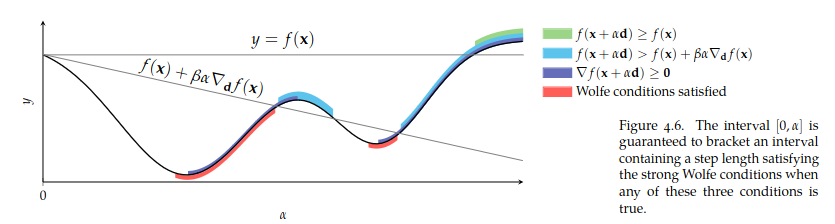
The condition for sufficient decreases is sometimes referred to as the first Wolfe condition. The second Wolfe condition, also known as the curvature condition, requires the directional derivative to be shallower each iteration:

$${\nabla }_{{\text{d}}^{(k)}}f({\text{x}}^{(k+1)})\ge \sigma {\nabla }_{{\text{d}}^{(k)}}f({\text{x}}^{(k)})$$

where $\gamma$ controls how shallow it needs to be. A common approach is $\beta <\sigma <1$. An alternative is the strong curvature condition:

$$|{\nabla }_{{\text{d}}^{(k)}}f({\text{x}}^{(k+1)})|\le -\sigma {\nabla }_{{\text{d}}^{(k)}}f({\text{x}}^{(k)})$$

Satisfying the strong Wolfe conditions can be done with strong backtracking line search. It begins by testing successively larger step sizes to bracket $[{\alpha }^{(k-1)},{\alpha }^{(k)}]$ so that it contains step lengths that satisfy Wolfe conditions, that is, it satisfies one of the following conditions

$$\begin{array}{rl}f(\text{x}+\alpha \text{d})& \ge f(\text{x})\\ f(\text{x}+\alpha \text{d})& \ge f(\text{x})+\beta \alpha {\nabla }_{\text{d}}f(\text{x})\\ \nabla f(\text{x}+\alpha \text{d})& \ge 0\end{array}$$

Next we enter the zoom phase where we shrink the interval to find a step size satisfying the strong Wolfe conditions via the bisection method.

Trust Region Methods

A trust region is a local area of the design space where the local model is believed to be reliable. In a trust region method we predict the improvement associated with taking a step (using line search), if the improvement closely matches the predicted value we expand the trust region. Otherwise, we contract the trust region.

This method is in the opposite order of line search methods by first choosing a maximum step size then the step direction. We find the next step parameters by minimizing a model of the objective function $\hat{f}$ over a trust region centered at the current design point $\text{x}$. A common choice is a second-order Taylor approximation. The radius of the trust region, $\delta$, is expanded and contracted as necessary. We then choose the next design point ${\text{x}}^{\prime }$ by solving

$$\begin{array}{rlr}& \underset{x}{\mathrm{minimize}}& \hat{f}({\text{x}}^{\prime })\\ & \text{subject to}& \Vert \text{x}-{\text{x}}^{\prime }\Vert \le \delta \end{array}$$

Termination Conditions

There are four common termination conditions:

• Maximum iterations: Terminate when $k$ exceeds some threshold $k_{\text{max}}$.
• Absolute Improvement: Terminate when the change in function value is less than some threshold

$$f({\text{x}}^{(k)})-f({\text{x}}^{(k+1)})<{ϵ}_a$$

• Relative Improvement: Similar to absolute improvement, but uses a threshold relative to the current function value

$$f({\text{x}}^{(k)})-f({\text{x}}^{(k+1)})<{ϵ}_r|f({\text{x}}^{(k)})|$$

• Gradient magnitude: Terminate when the function gradient is below a certain threshold

$$\Vert \nabla f({\text{x}}^{(k+1)})\Vert <{ϵ}_g$$