The structure and stability of persistence modules

Questions:

• ”…$T$ is a locally finite subset of $\mathbb{R}$…”
  • Answer: A locally finite poset is a poset $P$ such that for all $x,y\in P$ the interval $[x,y]=\{z\in P\mid x\le z\le y\}$ is finite. (https://en.wikipedia.org/wiki/Locally_finite_poset)
• Homology of sublevel sets
  • Answer: 2024-08-23
• Computing multiplicity, e,g, $⟨{\circ }_a\text{—}{\bullet }_b\text{—}{\bullet }_c\mid \mathbb{V}⟩$, without knowing the interval decomposition.
• Counterexample by Webb in Theorem 1.4 on page 13.
• Proof for Theorem 3.5.

Full paper can be found at: https://arxiv.org/abs/1207.3674

Smaller summary can be found at: 2024-08-30

An interleaving is an approximate isomorphism between two persistence modules. Moreover, the isometry theorem states that the interleaving distance is equal to the bottleneck distance under the assumption that the persistence modules are $q$-tame. A more general theorem is provided that does not depend on tameness.

Multisets

Persistence diagrams are multisets. We can think of a multiset as a pair $A=(S,m)$ where $S$ is the set and $m:S\to \mathbb{N}\cup \{\infty \}$ is the multiplicity of each element in $S$.

• The cardinality of $A=(S,m)$ is the sum

$$\text{card}A=\sum _{s\in S}m(s)$$

• We can restrict a multiset $A$ to a set $B$:

$$A{|}_B=(S\cap B,m{|}_{S\cap B})$$

• A pair $(B,m)$ with $m:B\to {\mathbb{N}}_0\cup \{\infty \}$ defines a multiset $A=(S,m{|}_S)$ where $S=B\backslash m^{-1}(0)$
• Given $f:S\to B$, the image $\{f(a)\mid a\in A\}$ is the multiset in $B$ with multiplicity

$$m^{\prime }(b)=\sum _{f^{-1}(b)}m(s)$$

Persistence Modules

All vector spaces are taken over an arbitrary field $k$.

Persistence module over a real parameter

A persistence module $\mathbb{V}$ over $\mathbb{R}$ is the indexed family of vector spaces $(V_t{)}_{t\in \mathbb{R}}$ with a family of linear maps $(v_s^t:V_s\to V_t\mid s\le t)$ such that $v_s^t\circ v_r^s=v_r^t$ whenever $r\le s\le t$ and $v_t^t={\text{id}}_{V_t}$.

One may replace $\mathbb{R}$ with any poset $T$. In such a case, we call $\mathbb{V}$ a $T$-persistence module. In practice, $T\subset \mathbb{R}$.

We can visualize this as a chain:

$$\cdots \to V_r\stackrel{v_r^s}{\to }{V}_s\stackrel{v_s^t}{\to }{V}_t\to \cdots$$

A classic example is sublevel sets:

$$X^t=(X,f{)}^t=\{x\in X\mid f(x)\le t\}$$

with inclusion maps

$$(i_s^t:X^s\hookrightarrow X^t\mid s\le t)$$

Functors from topological spaces to vector spaces also give rise to persistence modules. For example the $p$-dimensional singular homology functor gives rise to the persistence module $\mathbb{V}$ composed of $V_t=H(X^t)$ with maps on homology $v_s^t=H(i_s^t):H(X^s)\to H(X^t)$ induced by the functor on inclusion maps.

Quite often our space $X$ is a finite simplicial complex and each $X^t$ forms a subcomplex. As $t$ increases there are finitely many ‘critical values’

$$H(X^{a_1})\to H(x^{a_2})\to \cdots \to H(x^{a_n})$$

As a result, they are often $q$-tame, i.e., $\text{rank}(v_s^t)<\infty$ whenever $s<t$. The map from $q$-tame persistence modules to persistence diagrams is an isometry, i.e., a distance-preserving transformation between metric spaces.

Category of Persistence Modules

Homomorphism between persistence modules

A homomorphism between two $T$-persistence modules $\mathbb{U},\mathbb{V}$ is a collection of linear maps

$({\varphi }_t:U_t\to V_t\mid t\in T)$

such that the diagram

commutes for all $s\le t$.

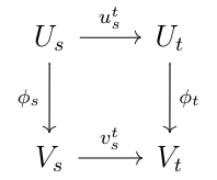
$T$-persistence modules with the above homomorphisms defines a category. The identity map ${\text{id}}_{\mathbb{V}}\in \text{Hom}(\mathbb{V},\mathbb{V})$ is the collection of identity maps $({\text{id}}_{V_t}:V_t\to V_t\mid t\in T)$. Composition is defined in the “obvious manner”, for $\Phi \in \text{Hom}(\mathbb{U},\mathbb{V})$ and $\Psi \in \text{Hom}(\mathbb{V},\mathbb{W})$ the composition $\Psi \Phi \in \text{Hom}(\mathbb{U},\mathbb{W})$ is the collection of composed linear maps $({\psi }_t{\varphi }_t:U_t\to W_t\mid t\in T)$.

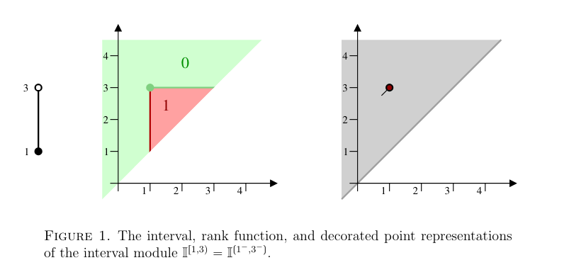
Interval Modules

Let $J\subset T\subset \mathbb{R}$ where $J$ is an interval. We define the $T$-persistence module ${\mathbb{I}}_T^J$ with spaces

$$I_t=\{\begin{array}{ll}k& \text{if }t\in J\\ 0& \text{otherwise}\end{array}$$

and maps

$$i_s^t=\{\begin{array}{ll}{\text{id}}_k& \text{if }s,t\in J\\ 0& \text{otherwise.}\end{array}$$

Example: Assume that $a<b<c$. Then the $\{a,b,c\}$-interval module ${\mathbb{I}}_{\{a,b,c\}}^{[a,b]}$ is the following persistence module:

$$k\stackrel{{\text{id}}_k}{\to }k\stackrel{0}{\to }0.$$

${\mathbb{I}}^J$ represents a feature that persists over an interval $J$ but is absent elsewhere. For example in homology groups, ${\mathbb{I}}^J$ may represent classes that persist over $J$ but are not present outside of $J$.

For $T=\mathbb{Z}$ there are four types of interval modules: ${\mathbb{I}}^{[m,n]}$, ${\mathbb{I}}^{(-\infty ,n]}$, ${\mathbb{I}}^{[m,\infty )}$, ${\mathbb{I}}^{(-\infty ,\infty )}$. Some sources write them as $\mathbb{I}[m,n]$ instead. However, over $\mathbb{R}$ two interval modules may have the same endpoints but with different topology, e.g., $\mathbb{I}(p,q]$ vs $\mathbb{I}(p,q)$.

Some sources use decorated real numbers:

• $(p^{-},q^{-})=[p,q)$
• $(p^{-},q^{+})=[p,q]$
• $(p^{+},q^{-})=(p,q)$
• $(p^{+},q^{+})=(p,q]$

If the decoration is unknown we use an asterisk $(p^{\ast },q^{\ast })$.

Interval modules can be visualized on the half-plane $\mathcal{H}=\{(p,q)\mid p\le q\}$. An interval module $\mathbb{I}(p^{\ast },q^{\ast })$ is either represented:

• as an interval on the real line
• as $\text{rank}(i_s^t)$, viewed as a function $\mathcal{H}\to \{0,1\}$
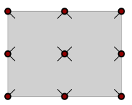
• as a point $(p,q)\in \mathcal{H}$ with a tick specifying the decoration. There are four possible tick directions:

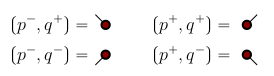The convention is that they point into the quadrant suggested by the decoration (This is unclear).

The classical persistence diagram draws points $(p,q)$ without indicating the decoration.

Interval Decomposition

Recall the direct sum of vector spaces. Given vector spaces $X$ and $Y$, the direct sum $X\oplus Y$ is the vector space $V=X+Y$ when $X\cap Y=\{0\}$. The direct sum is isomorphic to the direct product, i.e., the vector space consisting of all ordered pairs $(x,y)$ with operations defined component wise:

• $(x_1,y_1)+(x_2,y_2)=(x_1+x_2,y_1+y_2)$
• $\alpha (x,y)=(\alpha x,\alpha y)$

Moreover, given two maps $T:X\to X^{\prime }$ and $S:Y\to Y^{\prime }$, we can create the map $T\oplus S:X\oplus Y\to X^{\prime }\oplus Y^{\prime }$ by defining it component wise

$$(T\oplus S)(x,y)=(T(x),S(y)).$$

We can then define the direct sum of persistence modules.

Direct Sum

Given two $T$-persistence modules $\mathbb{U},\mathbb{V}$, the direct sum $\mathbb{W}=\mathbb{U}\oplus \mathbb{V}$ consists of the vector spaces $(W_t=U_t\oplus V_t\mid t\in T)$ with linear maps $(w_s^t=u_s^t\oplus v_s^t\mid s\le t).$

An alternative viewpoint is we are decomposing a persistence module $\mathbb{W}$ into smaller persistence modules $\mathbb{U}$ and $\mathbb{V}$. We say a persistence module is indecomposable if the only decompositions are the trivial $\mathbb{W}=\mathbb{W}\oplus 0$ or $\mathbb{W}=0\oplus \mathbb{W}$.

Our goal is decompose a persistence module $\mathbb{V}$ into an indexed family of interval modules:

$$\mathbb{V}=\underset{\ell \in L}{⨁}{\mathbb{I}}^{J_{\ell }}.$$

This is a generalization of what we do with homology groups. For example, if we have filtration of a simplicial complex

$$K_1\hookrightarrow K_2\hookrightarrow \cdots \hookrightarrow K_n$$

then we obtain a persistence module $\mathbb{V}=(H_i(K_j){)}_j$ with linear maps induced by inclusion

$$H_i(K_1)\to H_i(K_2)\to \cdots \to H_i(K_n).$$

This persistence module then decomposes into a persistence module formed by interval modules

$${\mathbb{Z}}_2^{k_1}\to {\mathbb{Z}}_2^{k_2}\cdots \to {\mathbb{Z}}_2^{k_n}.$$

Proposition 1.1

Let $\mathbb{I}$ be an interval module over $I\subset \mathbb{R}$. Then $\text{Hom}(\mathbb{I},\mathbb{I})=k$.

Proof: Let $\Phi \in \text{Hom}(\mathbb{I},\mathbb{I})$. Then each ${\varphi }_t\in \Phi$ is an endomorphism on 0 or $k$. In the non-trivial case, ${\varphi }_t(x)={\alpha }_{t}x$ is the only possible endomorphism. Notice that for all $s\le t$

$${\varphi }_t{u}_s^t(x)={\varphi }_t(x){\text{id}}_k={\alpha }_{t}x$$

and

$$v_s^t{\varphi }_s(x)={\text{id}}_k{\varphi }_s(x)={\alpha }_{s}x.$$

But ${\varphi }_t{u}_s^t=v_s^t{\varphi }_s$. Therefore, ${\varphi }_t={\varphi }_s$.

Q.E.D.

Proposition 1.2

Interval modules are indecomposable.

Proof: Assume that $\mathbb{I}=\mathbb{U}\oplus \mathbb{V}$. Notice that the projection map $(u,v)\mapsto (u,0)$ is idempotent, i.e., $f(f(x))=f(x)$, in $\text{Hom}(\mathbb{I},\mathbb{I})$. From the previous proof we know that the only idempotent endomorphisms are 0 and ${\text{id}}_k$. Therefore, the projection map is either trivial or an isomorphism.

Q.E.D.

Theorem 1.3 (Krull-Remak-Schmidt-Azumaya)

Suppose that a $T$-persistence module $\mathbb{V}$ decomposes in two ways:

$$\mathbb{V}=\underset{\ell \in L}{⨁}{\mathbb{I}}^{J_{\ell }}=\underset{m\in M}{⨁}{\mathbb{I}}^{K_m}.$$

Then there is a bijection $\sigma :L\to M$ such that $J_{\ell }=K_{\sigma (m)}$ for all $\ell \in L$.

In other words, decomposing a $T$-persistence module into interval modules is unique up to order.

Theorem 1.4 (Gabriel, Auslander, Ringel-Tachikawa, Webb)

Let $\mathbb{V}$ be a persistence module over $T\subset \mathbb{R}$. Then $\mathbb{V}$ can be decomposed as a direct sum of interval modules if

1. $T$ is a finite set; or
2. $T$ is a locally finite subset of $\mathbb{R}$ and each $V_t$ is finite-dimensional.

If either condition (1) or condition (2) in the above theorem hold, we can define a persistence diagram. However, we then see that not every persistence module over $\mathbb{R}$ is guaranteed an interval decomposition. For example, consider the following (from Webb) persistence module over the non-positive integers:

$$\begin{array}{rlrl}{V}_0& =\{\text{sequences (x1,x2,x3,…) of real numbers}\}& & \\ V_{-n}& =\{\text{sequences with x1=⋯=xn=0}\}& & n\ge 1\end{array}$$

with maps $v_{-m}^{-n}$ given by inclusion $V_{-m}\hookrightarrow V_{-n}$ for $m\ge n$.

$$\cdots \hookrightarrow V_{-3}\hookrightarrow V_{-2}\hookrightarrow V_{-1}\hookrightarrow V_0$$

Suppose $\mathbb{V}$ has an interval decomposition. Every map $v_{-n-1}^{-n}$ is injective so each interval is of the form $[-n,0]$ or $(-\infty ,0]$. Moreover, $\bigcap V_{-n}=\{(0,0,\dots )\}$ implying that the interval $(-\infty ,0]$ does not occur. Hence, $\mathbb{V}\cong {⨁}_{n\ge 0}\mathbb{I}[-n,0]$. But $\dim (V_0)$ is uncountable, a contradiction.

If conditions (1) and (2) are not satisfied, one may

• Work in restricted settings so that $\mathbb{V}$ only depends on finitely many indices $t\in \mathbb{R}$,
• Sample the persistence module over a finite grid, or
• Show that the persistence intervals can be inferred from the behavior of $\mathbb{V}$ on finite index sets.

The persistence diagram of a decomposable module

(Un)decorated persistence diagram

If a persistence module $\mathbb{V}$ can be decomposed as

$$\mathbb{V}\cong \underset{\ell \in L}{⨁}\mathbb{I}(p_{\ell }^{\ast },q_{\ell }^{\ast }),$$

then we define the decorated persistence diagram to be the multiset

$$\text{Dgm}(\mathbb{V})=\text{Int}(\mathbb{V})=\{(p_{\ell }^{\ast },q_{\ell }^{\ast })\mid \ell \in L\}$$

and the undecorated persistence diagram as the multiset

$$\text{dgm}(\mathbb{V})=\text{int}(\mathbb{V})=\{(p_{\ell },q_{\ell })\mid \ell \in L\}\setminus \Delta$$

where $\Delta =\{(r,r)\mid r\in \mathbb{R}\}$ is the diagonal in the plane.

The persistence diagram does not depend on the order of interval modules in the decomposition (see Theorem 1.3).

Example:

Consider the curve in ${\mathbb{R}}^2$ below filtered by height:

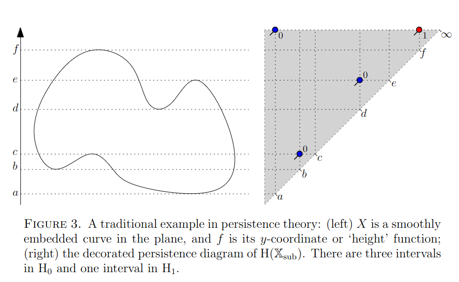
The sublevelset persistent homology decomposes as follows:

$$H_0({\mathbb{X}}_{\text{sub}})\cong \mathbb{I}(a^{-},\infty )\oplus \mathbb{I}(b^{-},c^{-})\oplus \mathbb{I}(d^{-},e^{-})$$ $$H_1({\mathbb{X}}_{\text{sub}})\cong \mathbb{I}(f^{-},\infty ).$$

Quiver calculations

Let $\mathbb{V}$ be a persistence module over a finite subset $\text{T}:a_1<a_2<\cdots <a_n$ of the real line. We may view $\mathbb{V}$ as a diagram of $n$ vector spaces and $n-1$ linear maps:

$$\mathbb{V}:V_{a_1}\to V_{a_2}\to \cdots \to V_{a_n}.$$

Such a diagram is a representation of the quiver

$$\bullet \to \bullet \to \cdots \to \bullet$$

For example, if $a<b<c$ then

$$\mathbb{I}[a,b]={\bullet }_a\text{—}{\bullet }_b\text{—}{\circ }_c$$

is the interval module over $\{a,b,c\}\subset \mathbb{R}$ given by $k\to k\to 0$. With quivers we use filled circles $\bullet$ where the module has rank 1 and open circles $\circ$ where the module has rank 0.

Multiplicity

Let $\mathbb{V}$ be a persistence module indexed over $\mathbb{R}$. If $\text{T}:a_1<a_2<\cdots <a_n$, then we define the multiplicity of $[a_i,a_j]\subseteq \text{T}$ in ${\mathbb{V}}_{\text{T}}$ to be the number of copies of $\mathbb{I}[a_i,a_j]$ in the interval decomposition of ${\mathbb{V}}_{\text{T}}$.

We write

$$⟨[b,c]\mid {\mathbb{V}}_{a,b,c}⟩\text{ or }⟨{\circ }_a\text{—}{\bullet }_b\text{—}{\bullet }_c\mid \mathbb{V}⟩$$

for the multiplicity of ${\circ }_a\text{—}{\bullet }_b\text{—}{\bullet }_c$ in the module

$${\mathbb{V}}_{a,b,c}=(V_a\to V_b\to V_c).$$

Given a linear map $V_a\stackrel{v}{\to }{V}_b$,

$$\begin{array}{rl}\text{rank}(v)& =⟨{\bullet }_a\text{—}{\bullet }_b\mid \mathbb{V}⟩\\ \text{nullity}(v)& =⟨{\bullet }_a\text{—}{\circ }_b\mid \mathbb{V}⟩\\ \text{conullity}(v)& =⟨{\circ }_a\text{—}{\bullet }_b\mid \mathbb{V}⟩\end{array}$$

The conullity is the dimension of the cokernel, for linear map $f:X\to Y$, the cokernel of $f$ is the quotient space $Y/\text{Im}(f)$.

Proposition 1.9 (direct sums)

Suppose $\mathbb{V}$ is the direct sum of persistence modules,

$$\mathbb{V}=\underset{\ell \in L}{⨁}{\mathbb{V}}^{\ell }.$$

Then

$$⟨[a_i,a_j]\mid {\mathbb{V}}_{\text{T}}⟩=\sum _{\ell \in L}⟨[a_i,a_j]\mid {\mathbb{V}}_{\text{T}}^{\ell }⟩$$

for any index set $\text{T}=\{a_1,a_2,\cdots ,a_n\}$ and interval $[a_i,a_j]\subset \text{T}$.

In other words, the multiplicity of $[a_i,a_j]$ in ${\mathbb{V}}_{\text{T}}$ is the sum of multiplicities of $[a_i,a_j]$ in each component.

Proposition 1.10 (restriction principle)

Let $\text{S}\subset \text{T}$ be finite index sets. Then

$$⟨\mathbb{I}\mid {\mathbb{V}}_{\text{S}}⟩=\sum _{\mathbb{J}}⟨\mathbb{J}\mid {\mathbb{V}}_{\text{T}}⟩$$

where the sum is over all intervals $\mathbb{J}\subseteq \text{T}$ which restrict over $\text{S}$ to $\mathbb{I}$.

Example: Let $a<b<c$ and consider new indices $p$ and $q$ such that $a<p<b<q<c$. Then

$$⟨{\circ }_a\text{—}{\bullet }_b\text{—}{\bullet }_c\mid {\mathbb{V}}_{a,b,c}⟩=⟨{\circ }_a\text{—}{\bullet }_b\text{—}{\bullet }_q\text{—}{\bullet }_c\mid {\mathbb{V}}_{a,b,q,c}⟩$$

and

$$⟨{\circ }_a\text{—}{\bullet }_b\text{—}{\bullet }_c\mid {\mathbb{V}}_{a,b,c}⟩=⟨{\circ }_a\text{—}{\circ }_p\text{—}{\bullet }_b\text{—}{\bullet }_c\mid {\mathbb{V}}_{a,p,b,c}⟩+⟨{\circ }_a\text{—}{\bullet }_p\text{—}{\bullet }_b\text{—}{\bullet }_c\mid {\mathbb{V}}_{a,p,b,c}⟩.$$

Notice the second term is due to both $\mathbb{J}[b,c]$ and $\mathbb{J}[p,c]$ both restricting to $\mathbb{I}[b,c]$.

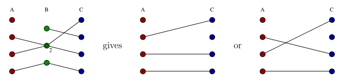
We can make use of proposition 1.10 to prove statements about ranks: Example: We wish to show that $\text{rank}(V_b\to V_c)\ge \text{rank}(V_a\to V_d)$ when $a\le b\le c\le d$. Notice that

$$\begin{array}{rl}\text{rank}(V_b\to V_c)& =⟨{\bullet }_b\text{—}{\bullet }_c\mid {\mathbb{V}}_{b,c}⟩\\ & =⟨{\bullet }_a\text{—}{\bullet }_b\text{—}{\bullet }_c\text{—}{\bullet }_d\mid {\mathbb{V}}_{a,b,c,d}⟩+⟨{\circ }_a\text{—}{\bullet }_b\text{—}{\bullet }_c\text{—}{\bullet }_d\mid {\mathbb{V}}_{a,b,c,d}⟩\\ & +⟨{\bullet }_a\text{—}{\bullet }_b\text{—}{\bullet }_c\text{—}{\circ }_d\mid {\mathbb{V}}_{a,b,c,d}⟩+⟨{\circ }_a\text{—}{\bullet }_b\text{—}{\bullet }_c\text{—}{\circ }_d\mid {\mathbb{V}}_{a,b,c,d}⟩\\ & \ge ⟨{\bullet }_a\text{—}{\bullet }_b\text{—}{\bullet }_c\text{—}{\bullet }_d\mid {\mathbb{V}}_{a,b,c,d}⟩\\ & =⟨{\bullet }_a\text{—}{\bullet }_d\mid {\mathbb{V}}_{a,d}⟩\\ & =\text{rank}(V_a\to V_d)\end{array}$$

Rectangle Measures

Right now our definitions for (un)decorated persistence diagrams requires knowing the interval module decomposition of our persistence module. We want a simpler methodology for constructing persistence diagrams. For that we use measure theory.

Persistence Measure

Let $\mathbb{V}$ be a persistence module. The persistence measure of $\mathbb{V}$ is the function

$${\mu }_{\mathbb{V}}(R)=⟨{\circ }_a\text{—}{\bullet }_b\text{—}{\bullet }_c\text{—}{\circ }_d\mid \mathbb{V}⟩$$

defined on rectangles $R=[a,b]\times [c,d]$ in the plane where $a<b\le c<d$.

That is, the persistence measure ${\mu }_{\mathbb{V}}$ is the number of copies of $\mathbb{I}[b,c]$ in the interval decomposition of ${\mathbb{V}}_{a,b,c,d}$.

This “measure” is easy to calculate on interval modules.

Proposition 2.1

Let $\mathbb{V}={\mathbb{I}}^J$ where $J=(p^{\ast },q^{\ast })$ is a real interval. Let $R=[a,b]\times [c,d]$ where $a<b\le c<d$. Then

$${\mu }_{\mathbb{V}}(R)=\{\begin{array}{ll}1& \text{if }[b,c]\subseteq J\subseteq (a,d)\\ 0& \text{otherwise.}\end{array}$$

Proof: Notice that ${\mu }_{\mathbb{V}}(R)=1$ when

$${\mathbb{I}}_{a,b,c,d}^J={\circ }_a\text{—}{\bullet }_b\text{—}{\bullet }_c\text{—}{\circ }_d$$

which occurs if and only if $b,c\in J$ and $a,d\notin J$.

Q.E.D.

Graphically we can determine when decorated point $(p^{\ast },q^{\ast })$ are detected by ${\mu }_{\mathbb{V}}(R)$:

• If $(p,q)$ is in the interior of $R$, then $(p^{\ast },q^{\ast })$ is always detected
• If $(p,q)$ is on the boundary, then $(p^{\ast },q^{\ast })$ is detected if the tick is pointed inwards.

Thus, we say that a decorated point $(p^{\ast },q^{\ast })\in R$ if the point $(p,q)$ and its decoration tick are contained in the closed rectangle $R$. This is equivalent to $[b,c]\subseteq (p^{\ast },q^{\ast })\subseteq (a,d)$. We denote the set of points in $R$ by

$$R^{■}:=\{(p^{\ast },q^{\ast })\in R\}.$$

Corollary 2.2

Suppose $\mathbb{V}$ is a decomposable persistence module over $\mathbb{R}$, then

$${\mu }_{\mathbb{V}}(R)=\text{card}(\text{Dgm}(\mathbb{V}){|}_R).$$

Proof: By Proposition 1.9 and 2.1,

$${\mu }_{\mathbb{V}}(R)={\mu }_{{⨁}_{\ell \in L}\mathbb{I}(p_{\ell }^{\ast },q_{\ell }^{\ast })}(R)=\sum _{\ell \in L}{\mu }_{\mathbb{I}(p_{\ell }^{\ast },q_{\ell }^{\ast })}(R)=\text{card}(\text{Dgm}(\mathbb{V}){|}_R)$$

Q.E.D.

With this we can layout the strategy for defining persistence diagrams without decomposing:

1. construct the persistence measure ${\mu }_{\mathbb{V}}$;
2. let $\text{Dgm}(\mathbb{V})$ be a multiset in the half-plane such that ${\mu }_{\mathbb{V}}(R)=\text{card}(\text{Dgm}(\mathbb{V}){|}_R)$ holds for all rectangles $R$.

Proposition 2.3

Let $\mathbb{V}$ be a persistence module and $a<b\le c<d$. If the spaces $V_a$, $V_b$, $V_c$, $V_d$ are finite-dimensional or $r_b^c=\text{rank}(v_b^c:V_b\to V_c)$, then

$$⟨{\circ }_a\text{—}{\bullet }_b\text{—}{\bullet }_c\text{—}{\circ }_d\mid \mathbb{V}⟩=r_b^c-r_a^c-r_b^d+r_a^d.$$

Proof: By the restriction principle:

$$\begin{array}{rlrlr}{r}_b^c& =⟨{\circ }_a\text{—}{\bullet }_b\text{—}{\bullet }_c\text{—}{\circ }_d⟩& +⟨{\bullet }_a\text{—}{\bullet }_b\text{—}{\bullet }_c\text{—}{\circ }_d⟩& +⟨{\circ }_a\text{—}{\bullet }_b\text{—}{\bullet }_c\text{—}{\bullet }_d⟩& +⟨{\bullet }_a\text{—}{\bullet }_b\text{—}{\bullet }_c\text{—}{\bullet }_d⟩\\ r_a^c& =& ⟨{\bullet }_a\text{—}{\bullet }_b\text{—}{\bullet }_c\text{—}{\circ }_d⟩& & +⟨{\bullet }_a\text{—}{\bullet }_b\text{—}{\bullet }_c\text{—}{\bullet }_d⟩\\ r_b^d& =& & ⟨{\circ }_a\text{—}{\bullet }_b\text{—}{\bullet }_c\text{—}{\bullet }_d⟩& +⟨{\bullet }_a\text{—}{\bullet }_b\text{—}{\bullet }_c\text{—}{\bullet }_d⟩\\ r_a^d& =& & & ⟨{\bullet }_a\text{—}{\bullet }_b\text{—}{\bullet }_c\text{—}{\bullet }_d⟩\end{array}$$

All the terms are finite.

Q.E.D.

Moreover, the measure is additive with respect to vertical or horizontal splitting of the rectangle:

Proposition 2.4

Whenever $a<p<b\le c<q<d$ we get that

$$\begin{array}{rl}{\mu }_{\mathbb{V}}([a,b]\times [c,d])& ={\mu }_{\mathbb{V}}([a,p]\times [c,d])+{\mu }_{\mathbb{V}}([p,b]\times [c,d])\\ {\mu }_{\mathbb{V}}([a,b]\times [c,d])& ={\mu }_{\mathbb{V}}([a,b]\times [c,q])+{\mu }_{\mathbb{V}}([a,b]\times [q,d])\end{array}$$

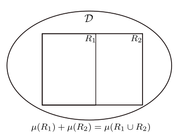
Proof: Notice that by direct calculation using the restriction principle

$$\begin{array}{rl}{\mu }_{\mathbb{V}}([a,b]\times [c,d])& =⟨{\circ }_a\text{—}{\bullet }_b\text{—}{\bullet }_c\text{—}{\circ }_d⟩\\ & =⟨{\circ }_a\text{—}{\bullet }_p\text{—}{\bullet }_b\text{—}{\bullet }_c\text{—}{\circ }_d⟩+⟨{\circ }_a\text{—}{\circ }_p\text{—}{\bullet }_b\text{—}{\bullet }_c\text{—}{\circ }_d⟩\\ & =⟨{\circ }_a\text{—}{\bullet }_p\text{—}{\bullet }_c\text{—}{\circ }_d⟩+⟨{\circ }_p\text{—}{\bullet }_b\text{—}{\bullet }_c\text{—}{\circ }_d⟩\\ & ={\mu }_{\mathbb{V}}([a,p]\times [c,d])+{\mu }_{\mathbb{V}}([p,b]\times [c,d]).\end{array}$$

A similar calculation follows for vertical splits.

Q.E.D.

Abstract r-measures

Rectangle Measure

Let $\mathcal{D}\subset {\mathbb{R}}^2$. Define

$$\text{Rect}(\mathcal{D})=\{[a,b]\times [c,d]\subset \mathcal{D}\mid a<b\text{ and }c<d\},$$

i.e., the set of closed rectangles that are contained in $\mathcal{D}$. A rectangle measure or r-measure on $\mathcal{D}$ is a function

$$\mu :\text{Rect}(\mathcal{D})\to \{0,1,2,\cdots \}\cup \{\infty \}$$

that is additive under vertical and horizontal splitting (satisfies Proposition 2.4).

The $r$-measure assigns each closed rectangle $R$ that lies inside of the dataset $\mathcal{D}$ either infinity or a non-negative integer such that splitting a rectangle does not change the total “area”.

Proposition 2.6

Let $\mu$ be an $r$-measure on $\mathcal{D}$. Then

1. (finitely additive) If $R=R_1\cup \cdots \cup R_k$ with disjoint interiors, then $\mu (R)=\mu (R_1)+\cdots +\mu (R_k)$.
2. (monotone) If $R\subseteq S$, then $\mu (R)\le \mu (S)$.

Proposition 2.7

If $R\in \text{Rect}(\mathcal{D})$ is such that $R\subseteq R_1\cup \cdots \cup R_k$ with each $R_i\in \text{Rect}(\mathcal{D})$, then

$$\mu (R)\le \mu (R_1)+\cdots +\mu (R_k).$$

Equivalence of measures and diagrams

There is a correspondence between $r$-measures and decorated diagrams.

Interior

The interior of $\mathcal{D}\subset {\mathbb{R}}^2$ is given by

$${\mathcal{D}}^{\circ }=\{(p,q)\mid \exists R\in \text{Rect}(\mathcal{D})\text{s.t.}(p,q)\in R^{\circ }\}.$$

where $R^{\circ }$ is the interior of the closed rectangle $R$. The r-interior of $\mathcal{D}$ is

$${\mathcal{D}}^{■}=\{(p^{\ast },q^{\ast })\mid \exists R\in \text{Rect}(\mathcal{D})\text{s.t.}(p^{\ast },q^{\ast })\in R\}.$$

The interior is defined similarly to interior in topology. A point is in the interior of $\mathcal{D}$ if we can put an open rectangle around the point that is contained inside of $\mathcal{D}$. For $r$-interior, the only difference is we also include the tick decorations of points.

Theorem 2.8 (The equivalence theorem)

Let $\mathcal{D}\subseteq {\mathbb{R}}^2$. There is a bijective correspondence between:

• Finite $r$-measures on $\mathcal{D}$ ($\mu (R)<\infty$ for all $R\in \text{Rect}(\mathcal{D})$.
• Locally finite multisets $A$ in ${\mathcal{D}}^{■}$ $(\text{card}(A{|}_R)<R$ for all $R\in \text{Rect}(\mathcal{D})$).

The measure $\mu$ corresponding to the multiset $A$ is related by the formula

$$\mu (R)=\text{card}(A{|}_R)$$

for every $R\in \text{Rect}(\mathcal{D})$.

The cardinality of $A{|}_R$ is given by

$$\mu (R)=\sum _{(p^{\ast },q^{\ast })\in R}m(p^{\ast },q^{\ast })$$

where $m:{\mathcal{D}}^{■}\to \{0,1,2,\dots \}$ is the multiplicity function for $A$. Essentially, the measure of a rectangle $R$ can be done by counting the number of decorated points that lie inside $R$.

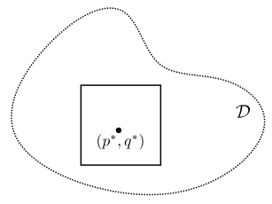
Proof Sketch:

• The correspondence from locally finite multisets $A$ in ${\mathcal{D}}^{■}$ to finite $r$-measures is given by the fact that $\mu (R)=\text{card}(A{|}_R)$ is a finite $r$-measure.
• The other direction: for $(p^{\ast },q^{\ast })\in {\mathcal{D}}^{■}$ define

$$m(p^{\ast },q^{\ast })=\min \{\mu (R)\mid R\in \text{Rect}(\mathcal{D}),(p^{\ast },q^{\ast })\in R\}.$$

• Use induction on $\mu (R)$ to show that

$$\nu (R)=\sum _{(p^{\ast },q^{\ast })\in R}m(p^{\ast },q^{\ast })=\mu (R).$$

- Base case ($\mu(R)=0$): $0\le m(p^*,q^*)\le\mu(R)=0$.
- Inductive step: split rectangle into four quadrants $R=S_1\cup\cdots\cup S_4$. Each quadrant satisfies $\mu(S_i)=\nu(S_i)$ by the inductive hypothesis. By finite additivity we get that $\nu(R)=\mu(R)$. If one of the quadrants has $\mu(S_i)=k$ then the rest have $\mu=0$. In such a case we repeat the subdivision on $S_i$. This either terminates or gives us a sequence of closed rectangles
$$
	R_0\supset R_1\supset\cdots
$$
- with each $\mu(R_i)=k$. The only contribution to $\nu(R)$ is then the decorated points $(p^*,q^*)$ that belong to each rectangle in the sequence.

• Show that if $\mu ={\nu }^{\prime }$ for some other multiplicity function $m^{\prime }$, then $m=m^{\prime }$.

This immediately results in the following definitions:

1. The decorated diagram of $\mu$ is the unique locally finite multiset $\text{Dgm}(\mu )$ in ${\mathcal{D}}^{■}$ such that

$$\mu (R)=\text{card}(\text{Dgm}(\mu ){|}_R)$$

for every $R\in \text{Rect}(\mathcal{D})$. 2. The undecorated diagram of $\mu$ is the locally finite multiset in ${\mathcal{D}}^{\circ }$

$$\text{dgm}(\mu )=\{(p,q)\mid (p^{\ast },q^{\ast })\in \text{Dgm}(\mu )\}\cap {\mathcal{D}}^{\circ }$$

obtained by forgetting the decorations and restricting to the interior.

Non-finite measures

We now consider the case where the $r$-measure is not finite.

Finite interior

The finite interior of an $r$-measure $\mu$ is given by

$${\mathcal{F}}^{\circ }(\mu )=\{(p,q)\mid \exists R\in \text{Rect}(\mathcal{D})\text{s.t.}(p,q)\in R^{\circ }\text{ and }\mu (R)<\infty \}.$$

The finite r-interior is then

$${\mathcal{F}}^{■}(\mu )=\{(p^{\ast },q^{\ast })\mid \exists R\in \text{Rect}(\mathcal{D})\text{s.t.}(p^{\ast },q^{\ast })\in R\text{ and }\mu (R)<\infty \}.$$

This is the same as interior and $r$-interior with the caveat that we now also require our rectangle to have finite measure.

We apply Theorem 2.8 (the equivalence theorem) to each rectangle $R$ with finite measure and get a decorated diagram in $R^{■}$. We then stitch together the local definitions to get the multiset $\text{Dgm}(\mu )$ in the entirety of ${\mathcal{F}}^{■}(\mu )$. This multiset satisfies

$$\mu (R)=\text{card}(\text{Dgm}(\mu ){|}_R)$$

for any rectangle $R\in \text{Rect}(\mathcal{D})$ with finite measure.

Proposition 2.14

Let $R\in \text{Rect}(\mathcal{D})$. If $R^{■}\subseteq {\mathcal{F}}^{■}(\mu )$, then $\mu (R)<\infty$.

Corollary 2.15

Let $\mu$ be an $r$-measure on $\mathcal{D}\subseteq {\mathbb{R}}^2$. Then there is a uniquely defined locally finite multiset $\text{Dgm}(\mu )$ in ${\mathcal{F}}^{■}(\mu )$ such that

$$\mu (R)=\text{card}(\text{Dgm}(\mu ){|}_R)$$

for every $R\in \text{Rect}(\mathcal{D})$ with $R^{■}\subseteq {\mathcal{F}}^{■}(\mu )$.

Proposition 2.14

Let $R\in \text{Rect}(\mathcal{D})$. If $R\subseteq {\mathcal{F}}^{\circ }(\mu )$, then $\mu (R)<\infty$.

Hence, we can define the diagrams for any general $r$-measure:

• The decorated diagram of an $r$-measure is the pair $(\text{Dgm}(\mu ),{\mathcal{F}}^{■}(\mu ))$, where $\text{Dgm}(\mu )$ is the multiset in ${\mathcal{F}}^{■}(\mu$)$ described in corollary 2.15
• The undecorated diagram is the pair $(\text{dgm}(\mu ),{\mathcal{F}}^{\circ }(\mu ))$, where

$$\text{dgm}(\mu )=\{(p,q)\mid (p^{\ast },q^{\ast })\in \text{Dgm}(\mu )\}\cap {\mathcal{F}}^{\circ }(\mu ).$$

The diagram at infinity

We focus on $r$-measures in the extended plane which now requires discussion of infinite rectangles.

The $r$-interior and interior of $\mathcal{D}$ remain primarily the same with the subtlety that now $R^{\circ }$ is the relative interior, e.g., if $R=[-\infty ,b]\times [c,d]$ with $b,c,d$ finite, then $R^{\circ }=[-\infty ,b)\times (c,d)$.

We define the singular support of $\mu$ as

$$\delta (\mu )={\overline{\mathbb{R}}}^2-{\mathcal{F}}^{\circ }(\mu ).$$

Corollary 2.15 still holds for $r$-measures in the extended plane. We can view ${\overline{\mathbb{R}}}^2$ as a rectangle in ${\mathbb{R}}^2$ via a transformation with homeomorphic embeddings, e.g.,

$$x^{\prime }=\arctan (x),y^{\prime }=\arctan (y)$$

identifies ${\overline{R}}^2$ with the rectangle $[-\pi /2,pi/2]\times [-\pi /2,\pi /2]$. Both Theorem 2.8 and Corollary 2.15 are invariant under such a transformation.

Let $\mathbb{V}$ be a persistence module. The persistence measure ${\mu }_{\mathbb{V}}$ previously defined by

$${\mu }_{\mathbb{V}}([a,b]\times [c,d])=⟨{\circ }_a\text{—}{\bullet }_b\text{—}{\bullet }_c\text{—}{\circ }_d\mid \mathbb{V}⟩$$

for $a<b\le c<d$ extends to infinite rectangles where $a=-\infty$ or $d=+\infty$ by setting $V_{-\infty }=V_{\infty }=0$. Such a choice gives us the k-triangle lemma:

$$\begin{array}{rlrlr}{\mu }_{\mathbb{V}}([-\infty ,b]\times [c,+\infty ])& =⟨{\bullet }_b\text{—}{\bullet }_c\mid \mathbb{V}⟩& =r_b^c& & \\ {\mu }_{\mathbb{V}}([a,b]\times [c,+\infty ])& =⟨{\circ }_a\text{—}{\bullet }_b\text{—}{\bullet }_c\mid \mathbb{V}⟩& =r_b^c-r_a^c& & (\text{if }{r}_a^c<\infty )\\ {\mu }_{\mathbb{V}}([-\infty ,b]\times [c,d])& =⟨{\bullet }_b\text{—}{\bullet }_c\text{—}{\circ }_d\mid \mathbb{V}⟩& =r_b^c-r_b^d& & (\text{if }{r}_b^d<\infty )\end{array}$$

One may view ${\mu }_{\mathbb{V}}$ as an $r$-measure on the extended half-plane

$$\overline{\mathcal{H}}=\{(p,q)\mid -\infty \le p\le q\le +\infty \}$$

and its diagram $\text{Dgm}({\mu }_{\mathbb{V}})$ is defined on the finite $r$-interior ${\overline{\mathcal{H}}}^{■}$.

Corollary 2.17

If $\mathbb{V}$ is decomposable into interval modules then ${\mu }_{\mathbb{V}}(R)$ counts the interval summands corresponding to decorated points which lie in $R$.

In other words, ${\mu }_{\mathbb{V}}(R)$ simply counts the number of decorated points that lie inside $R$.

There are three cases of relevance for the ‘measure at infinity’:

• the line $(-\infty ,\mathbb{R})$:

$$\mu (-\infty ,[c,d])=\underset{b\to -\infty }{\lim }\mu ([-\infty ,b]\times [c,d])=\underset{b}{\min }\mu ([-\infty ,b]\times [c,d])$$

• the line $(\mathbb{R},+\infty )$:

$$\mu ([a,b],+\infty )=\underset{c\to +\infty }{\lim }\mu ([a,b]\times [c,+\infty ])=\underset{c}{\min }\mu ([a,b]\times [c,+\infty ])$$

• the point $(-\infty ,+\infty )$:

$$\mu (-\infty ,+\infty )=\underset{e\to +\infty }{\lim }\mu ([-\infty ,-e]\times [e,+\infty ])=\underset{e}{\min }\mu ([-\infty ,-e]\times [e,+\infty ])$$

The above limits exist when the rectangles in the expression belong to $\text{Rect}(\mathcal{D})$.

Diagrams of persistence modules

We have defined two definitions of diagrams of persistence module:

• Decomposition of intervals $\mathbb{V}={⨁}_{\ell \in L}\mathbb{I}(p_{\ell }^{\ast },q_{\ell }^{\ast })$ gives the multiset

$$\text{Dgm}(\mathbb{V})=\text{Int}(\mathbb{V})=\{(p_{\ell }^{\ast },q_{\ell }^{\ast })\mid \ell \in L\}$$

• For persistence measure ${\mu }_{\mathbb{V}}$ of $\mathbb{V}$ gives the multiset that satisfies

$${\mu }_{\mathbb{V}}(R)=\text{card}(\text{Dgm}({\mu }_{\mathbb{V}}){|}_R)$$

for all rectangles $R$.

Proposition 2.18

If $\mathbb{V}$ is decomposable into intervals, then $\text{Int}(\mathbb{V})$ agrees with $\text{Dgm}({\mu }_{\mathbb{V}})$ where the latter is defined on ${\mathcal{F}}^{■}(\mu )$.

Example 2.19: Let

$$\mathbb{V}=\underset{\ell \in L}{⨁}\mathbb{I}(p_{\ell }^{\ast },q_{\ell }^{\ast })$$

where the undecorated pairs $(p_{\ell },q_{\ell })$ form a dense subset of the half-plane $\overline{\mathcal{H}}$. Notice that that for any rectangle $R$, ${\mu }_{\mathbb{V}}(R)=\infty$ because the pairs are dense, i.e., there are infinitely many points in every rectangle. Hence,

$${\mathcal{F}}^{■}({\mu }_{\mathbb{V}})=\{(p^{\ast },q^{\ast })\mid \exists R\in \text{Rect}(\mathcal{D})\text{ s.t. }(p^{\ast },q^{\ast })\in R\text{ and }\mu (R)<\infty \}=\varnothing .$$

Therefore, the multiset $\text{Dgm}({\mu }_{\mathbb{V}})$ is nowhere defined.

Example 2.20: Consider the persistence module

$$\cdots \to W_{-2}\to W_{-1}\to W_0\to 0\to \cdots$$

defined by

$$\begin{array}{rlr}{W}_t& =0& \text{for }t>0\\ W_0& =\{\text{sequences (x1,x2,x3,…) of real numbers}\}& \\ W_t& =\{\text{sequences with xn=0 for all n≤∣t∣}\}& \text{for }t<0\end{array}$$

???

Tameness Conditions

We say a persistence module $\mathbb{V}$ is of finite type if it is a finite direct sum of interval modules. It is locally finite, if it is a direct sum of interval modules such that every $t\in \mathbb{R}$ has a neighborhood which meets only finitely many of the intervals.

Proposition 2.21

A persistence module $\mathbb{V}$ is locally finite if and only if

1. each $V_t$ is finite-dimensional
2. there is a locally finite set $S\subset \mathbb{R}$ such that $v_b^c$ is an isomorphism for every pair $b<c$ with $[b,c]\cap S=\varnothing$.

Condition (2) asserts that $\mathbb{V}$ is constant over each interval of the open set $\mathbb{R}\setminus S$.

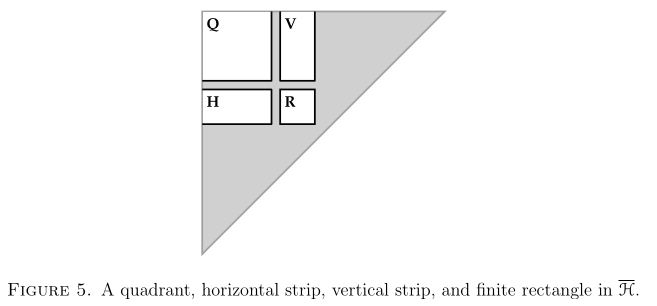
There are four kinds of tameness relating to the measure of various types of rectangles in $\overline{\mathcal{H}}$:

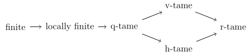
1. We say $\mathbb{V}$ is q-tame if ${\mu }_{\mathbb{V}}(Q)<\infty$ for every quadrant $Q$ (infinite rectangle) not touching the diagonal, i.e.,

$$\text{rank}(V_b\to V_c)=⟨{\bullet }_b\text{—}{\bullet }_c\mid \mathbb{V}⟩<\infty$$

for all $b<c$.

2. We say $\mathbb{V}$ is h-tame if ${\mu }_{\mathbb{V}}(H)<\infty$ for every horizontally infinite strip $H$ not touching the diagonal, i.e.,

$$⟨{\bullet }_b\text{—}{\bullet }_c\text{—}{\circ }_d\mid \mathbb{V}⟩<\infty$$

for all $b<c<d$.

3. We say $\mathbb{V}$ is v-tame if ${\mu }_{\mathbb{V}}(V)<\infty$ for every vertically infinite strip $V$ not touching the diagonal, i.e.,

$$⟨{\circ }_a\text{—}{\bullet }_b\text{—}{\bullet }_c\mid \mathbb{V}⟩<\infty$$

for all $a<b<c$.

4. We say $\mathbb{V}$ is r-tame if ${\mu }_{\mathbb{V}}(R)<\infty$ for every finite rectangle $R$ not touching the diagonal, i.e.,

$$⟨{\circ }_a\text{—}{\bullet }_b\text{—}{\bullet }_c\text{—}{\circ }_d\mid \mathbb{V}⟩<\infty$$

for all $a<b<c<d$.

One may show that

$$\text{q-tame}⊊\text{h-tame }\cap \text{ v-tame},\text{h-tame }\cup \text{ v-tame}⊊\text{r-tame}.$$

and the following diagram of inclusion:

Interleaving

Two persistence modules $\mathbb{U},\mathbb{V}$ are said to be isomorphic if there are maps

$$\Phi \in \text{Hom}(\mathbb{U},\mathbb{V}),\Psi \in \text{Hom}(\mathbb{V},\mathbb{U})$$

such that

$$\Psi \Phi =1_{\mathbb{U}},\Phi \Psi =1_{\mathbb{V}}.$$

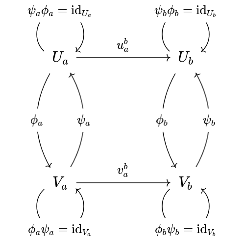
Such a relation is too strong to be used in practice. Instead we introduce a weaker relation known as $\delta$-interleaving where $\delta \ge 0$ quantifies a level of uncertainty.

Shifted Homomorphisms

Let $\mathbb{U},\mathbb{V}$ be persistence modules over $\mathbb{R}$ and $\delta \in \mathbb{R}$. A homomorphism of degree $\delta$ is a collection $\Phi$ of linear maps

$${\varphi }_t:U_t\to V_{t+\delta }$$

for all $t\in \mathbb{R}$ such that the diagram

commutes whenever $a\le b$.

We denote the set of homomorphisms $\mathbb{U}\to \mathbb{V}$ of degree $\delta$ by ${\text{Hom}}^{\delta }(\mathbb{U},\mathbb{V})$. One may compose two homomorphisms of degree ${\delta }_1$ and ${\delta }_2$ to get a homomorphism of degree ${\delta }_1+{\delta }_2$.

For $\delta \ge 0$ a crucial degree-$\delta$ endomorphism is the shift map $1_{\mathbb{V}}^{\delta }\in {\text{Hom}}^{\delta }(\mathbb{V},\mathbb{V})$ that is given by the collection of maps $(v_t^{t+\delta }:V_t\to V_{t+\delta }{)}_t$ from the underlying persistence structure on $\mathbb{V}$. This map satisfies

$$\Phi 1_{\mathbb{U}}^{\delta }=1_{\mathbb{V}}^{\delta }\Phi$$

for any $\Phi \in {\text{Hom}}^{\delta }(\mathbb{U},\mathbb{V})$ and $\delta \ge 0$, i.e., the diagram below commutes for all $t$ and $\delta \ge 0$.

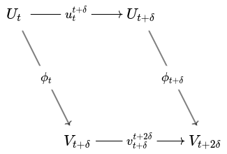
Interleaving

Two persistence modules $\mathbb{U},\mathbb{V}$ are said to be $\delta$-interleaved if there are maps

$$\Phi \in {\text{Hom}}^{\delta }(\mathbb{U},\mathbb{V}),\Psi \in {\text{Hom}}^{\delta }(\mathbb{V},\mathbb{U})$$

such that

$$\Psi \Phi =1_{\mathbb{U}}^{2\delta },\Phi \Psi =1_{\mathbb{V}}^{2\delta },$$

in other words, for all $a<b$ the diagrams below commute:

Example 3.2. Let $X$ be a topological space and let $f,g:X\to \mathbb{R}$. Suppose $\Vert f-g{\Vert }_{\infty }<\delta$. Then the persistence modules $H({\mathbb{X}}_{\text{sub}}^f)$ and $H({\mathbb{X}}_{\text{sub}}^g)$ are $\delta$-interleaved by the homomorphisms of degree $\delta$

$$\Phi :H({\mathbb{X}}_{\text{sub}}^f)\to H({\mathbb{X}}_{\text{sub}}^g),\Psi :H({\mathbb{X}}_{\text{sub}}^g)\to H({\mathbb{X}}_{\text{sub}}^f)$$

induced by inclusion

$$(X,f{)}^t\hookrightarrow (X,g{)}^{t+\delta },(X,g{)}^t\hookrightarrow (X,f{)}^{t+\delta }.$$

An interleaving between two persistence modules can be viewed as a persistence module over a poset. Consider the standard partial order on ${\mathbb{R}}^2$:

$$(p_1,q_1)\le (p_2,q_2)\iff p_1\le p_2\text{ and }{q}_1\le q_2.$$

Then for any $x\in \mathbb{R}$ we define the poset

$${\Delta }_x=\{(p,q)\mid q-p=2x\}\subset {\mathbb{R}}^2$$

that is isomorphic to $\mathbb{R}$ by $t\mapsto (t-x,t+x)$.

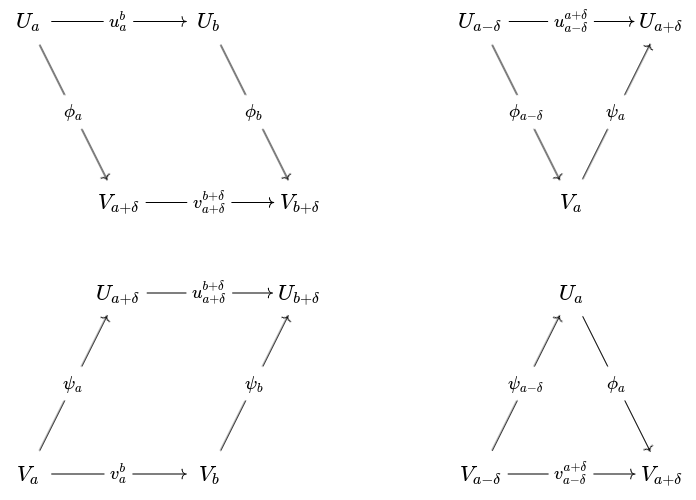
Proposition 3.3

Let $x,y\in \mathbb{R}$. Persistence modules $\mathbb{U},\mathbb{V}$ are $|y-x|$-interleaved if and only if there is a persistence module $\mathbb{W}$ over ${\Delta }_x\cup {\Delta }_y$ such that $\mathbb{W}{|}_{{\Delta }_x}=\mathbb{U}$ and $\mathbb{W}{|}_{{\Delta }_y}=\mathbb{V}$.

For $x=1$ and $y=2$, we may visualize $\mathbb{W}$ as follows:

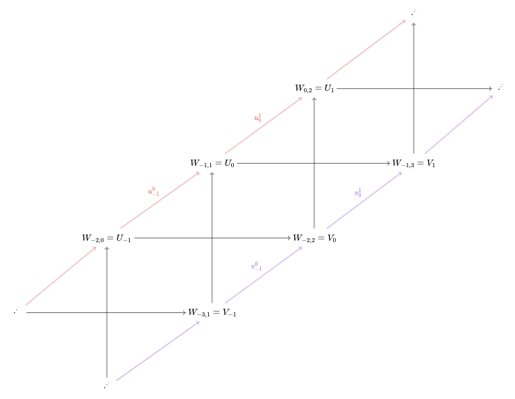
Proof: Assume WLOG that $x<y$.

1. Since $\mathbb{U},\mathbb{V}$ are $(y-x)$-interleaved, there are $(y-x)$-degree homomorphisms

$$\begin{array}{rl}\Phi & =({\varphi }_t:U_t\to V_{t+y-x}{)}_t\\ \Psi & =({\psi }_t:V_t\to U_{t+y-x}{)}_t\end{array}$$

such that for all $\eta \ge 0$

$$\Phi 1_{\mathbb{U}}^{\eta }=1_{\mathbb{V}}^{\eta }\Phi ,\Psi 1_{\mathbb{V}}^{\eta }=1_{\mathbb{U}}^{\eta }\Psi ,\Psi \Phi =1_{\mathbb{U}}^{2y-2x},\Phi \Psi =1_{\mathbb{V}}^{2y-2x}.$$

2. The persistence module $\mathbb{W}$ maps satisfy

$$w_R^T=w_S^T\circ w_R^S$$

for all $R\le S\le T$ in ${\Delta }_x\cup {\Delta }_y$. Notice that

$$\begin{array}{r}{\varphi }_t:U_t=W_{t-x,t+x}\to W_{t-x,t+2y-x}=V_{t+y-x}\\ {\psi }_t:V_t=W_{t-y,t+y}\to W_{t+y-2x,t+y}=U_{t+y-x}\end{array}$$

by the isomorphism $t\mapsto (t-x,t+x)$ for $\mathbb{R}\cong {\Delta }_x$. Moreover all maps $w_S^T$, where $S\le T$, in $\mathbb{W}$ can be factored as

$$\begin{array}{rl}{w}_S^T& =v_{s+y-x}^t\circ {\varphi }_s\text{if }S\in {\Delta }_x\text{ and }T\in {\Delta }_y\\ w_S^T& =u_{s+y-x}^t\circ {\psi }_s\text{if }S\in {\Delta }_y\text{ and }T\in {\Delta }_x.\end{array}$$

So every map in $\mathbb{W}$ is of the form

$$\begin{array}{rlr}& 1_{\mathbb{U}}^{\eta }& \text{from Δx to Δx}\\ & 1_{\mathbb{V}}^{\eta }& \text{from Δy to Δy}\\ & 1_{\mathbb{V}}^{\eta }\Phi & \text{from Δx to Δy}\\ & 1_{\mathbb{U}}^{\eta }\Psi & \text{from Δy to Δx}\end{array}$$

One may then show that the composition law is satisfied.

Q.E.D.

The Interpolation Lemma

Given two $\delta$-interleaved persistence modules $\mathbb{U}$ and $\mathbb{V}$, we can find a family of persistence modules that “continuously” transforms between $\mathbb{U}$ and $\mathbb{V}$.

Lemma 3.4 (Interpolation Lemma)

Suppose $\mathbb{U},\mathbb{V}$ are a $\delta$-interleaved pair of persistence modules. Then there exists a 1-parameter family of persistence modules $({\mathbb{U}}_x\mid x\in [0,\delta ])$ such that ${\mathbb{U}}_0,{\mathbb{U}}_{\delta }$ are equal to $\mathbb{U},\mathbb{V}$ respectively, and ${\mathbb{U}}_x,{\mathbb{U}}_y$ are $|y-x|$-interleaved for all $x,y\in [0,\delta ]$.

More specifically, given interleaving $\Phi \in {\text{Hom}}^{\delta }(\mathbb{U},\mathbb{V})$ and $\Psi \in {\text{Hom}}^{\delta }(\mathbb{V},\mathbb{U})$, then for each $x<y$ we get a pair of interleaving maps

$$\begin{array}{r}{\Phi }_x^y\in {\text{Hom}}^{y-x}({\mathbb{U}}_x,{\mathbb{U}}_y)\\ {\Psi }_y^x\in {\text{Hom}}^{y-x}({\mathbb{U}}_y,{\mathbb{U}}_x)\end{array}$$

such that ${\Phi }_0^{\delta }=\Phi$, ${\Psi }_{\delta }^0=\Psi$ and

$${\Phi }_x^z={\Phi }_y^z{\Phi }_x^y\text{ and }{\Psi }_z^x={\Psi }_y^x{\Psi }_z^y$$

for all $x<y<z$.

In other words, we get a persistence module.

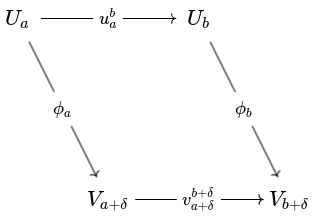
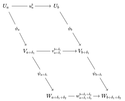
Theorem 3.5

Any persistence module $\mathbb{W}$ over ${\Delta }_0\cup {\Delta }_{\delta }$ extends to a persistence module $\overline{\mathbb{W}}$ over the diagonal strip

$${\Delta }_{[0,\delta ]}=\{(p,q)\mid 0\le q-p\le 2\delta \}\subset {\mathbb{R}}^2.$$

Proof Outline: We replace the interval $[0,\delta ]$ with $[-1,1]$ by rescaling and translating the plane. By proposition 3.3, the persistence module $\mathbb{W}$ satisfies $\mathbb{U}=\mathbb{W}{|}_{{\Delta }_{-1}}$ and $\mathbb{V}=\mathbb{W}{|}_{{\Delta }_1}$ which we view as persistence modules over $\mathbb{R}$:

$$\begin{array}{rl}{U}_t& =W_{(t+1,t-1)}\\ V_t& =W_{(t-1,t+1)}.\end{array}$$

We also get interleaving maps $\Phi \in {\text{Hom}}^2(\mathbb{U},\mathbb{V})$ and $\Psi \in {\text{Hom}}^2(\mathbb{V},\mathbb{U})$ of degree 2. We construct four persistence modules over ${\mathbb{R}}^2$:

$$\begin{array}{rl}\mathbb{A}& =\mathbb{U}[p-1]\text{ defined by }{A}_{(p,q)}=U_{p-1}\text{ and }{a}_{(p,q)}^{(r,s)}=u_{p-1}^{r-1}\\ \mathbb{B}& =\mathbb{V}[q-1]\text{ defined by }{B}_{(p,q)}=V_{q-1}\text{ and }{b}_{(p,q)}^{(r,s)}=v_{q-1}^{s-1}\\ \mathbb{C}& =\mathbb{U}[q+1]\text{ defined by }{C}_{(p,q)}=U_{q+1}\text{ and }{c}_{(p,q)}^{(r,s)}=u_{q+1}^{s+1}\\ \mathbb{D}& =\mathbb{V}[p+1]\text{ defined by }{D}_{(p,q)}=V_{p+1}\text{ and }{d}_{(p,q)}^{(r,s)}=v_{p+1}^{r+1}\end{array}$$

and module maps

$$\begin{array}{rl}{1}_{\mathbb{U}}& :\mathbb{A}\to \mathbb{C}\text{ defined at (p,q) to be }{u}_{p-1}^{q+1}:U_{p-1}\to U_{q+1}\\ \Phi & :\mathbb{A}\to \mathbb{D}\text{ defined at (p,q) to be }{\varphi }_{p-1}:U_{p-1}\to V_{p+1}\\ \Psi & :\mathbb{B}\to \mathbb{C}\text{ defined at (p,q) to be }{\psi }_{q-1}:V_{q-1}\to U_{q+1}\\ 1_{\mathbb{V}}& :\mathbb{B}\to \mathbb{D}\text{ defined at (p,q) to be }{v}_{q-1}^{p+1}:V_{q-1}\to V_{p+1}\end{array}$$

For example, if $\delta =0.5$:

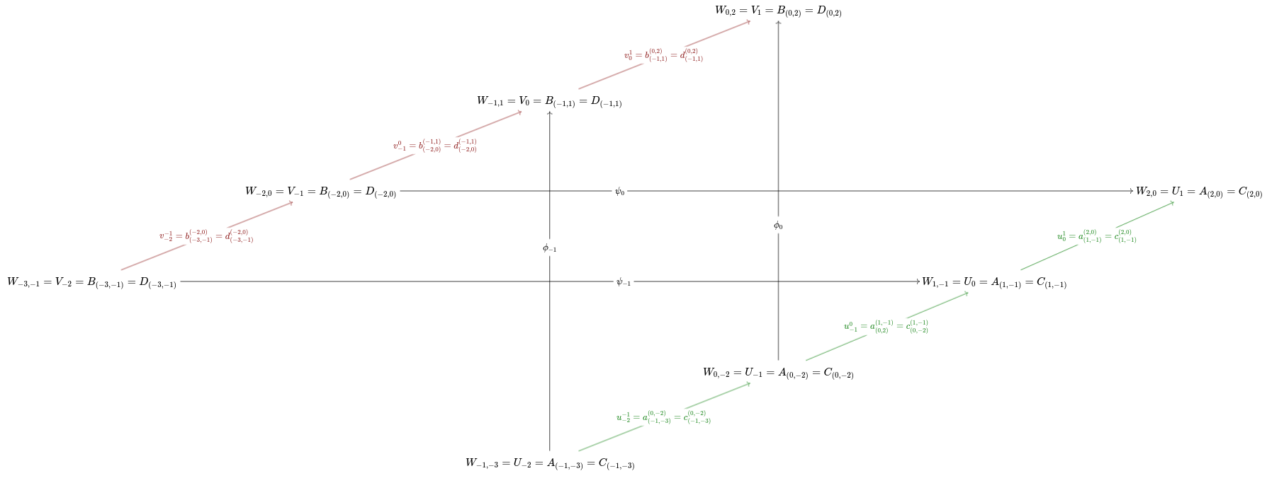
Define $\Omega \in \text{Hom}(\mathbb{A}\oplus \mathbb{B},\mathbb{C}\oplus \mathbb{D})$ by the 2-by-2 matrix

$$\left[\begin{array}{cc}{1}_{\mathbb{U}}& \Psi \\ \Phi & 1_{\mathbb{V}}\end{array}\right]$$

of module maps. We claim $\overline{\mathbb{W}}=\text{Im}(\Omega )$ is the desired extension.

1. $\overline{\mathbb{W}}{|}_{{\Delta }_{-1}}$ is isomorphic to $\mathbb{U}$.
2. ${\overline{\mathbb{W}}}_{{\Delta }_1}$ is isomorphic to $\mathbb{V}$.
3. The cross maps of $\overline{\mathbb{W}}$ are precisely $\Phi$ and $\Psi$.

The Interpolation Lemma (continued)

The Isometry Theorem

The main result is thaanks to Cohen-Steiner, Edelsbrunner and Harer in a 2007 paper.

The Interleaving Distance

Let $\mathbb{U}$ and $\mathbb{V}$ be $\delta$-interleaved. Then for every $ϵ>0$, they are $(\delta +ϵ)$-interleaved by the maps

$$\begin{array}{rl}{\Phi }^{\prime }& =\Phi 1_{\mathbb{U}}^{ϵ}=1_{\mathbb{V}}^{ϵ}\mathbb{V}\\ {\Psi }^{\prime }& =\Psi 1_{\mathbb{V}}^{ϵ}=1_{\mathbb{U}}^{ϵ}\mathbb{U}.\end{array}$$

We want to make the interleaving parameter as small as possible. We may not be able to attain the actual minimum.

We say that $\mathbb{U}$ and $\mathbb{V}$ are ${\delta }^{+}$-interleaved if they are $(\delta +ϵ)$-interleaved for all $ϵ>0$.

Example 4.1. Two persistence modules are isomorphic if and only if they are $0$-interleaved.

Example 4.2. Let $\mathbb{U}$ and $\mathbb{V}$ be two non-isomorphic ephemeral modules ($v_s^t=0$ for all $s<t$). Then $\mathbb{U},\mathbb{V}$ are $0^{+}$-interleaved but not 0-interleaved. Since $1_{\mathbb{U}}^{2ϵ}=0$ and $1_{\mathbb{V}}^{2ϵ}=0$ for all $ϵ>0$, it follows that the zero maps $\Phi =0$ and $\Psi =0$ are an $ϵ$-interleaving.

We define the interleaving distance between two persistence modules as

$$\begin{array}{rl}{d}_i(\mathbb{U},\mathbb{V})& =\inf \{\delta \mid \mathbb{U},\mathbb{V}\text{ are δ-interleaved}\}\\ & =\min \{\delta \mid \mathbb{U},\mathbb{V}\text{ are δ+-interleaved}\}.\end{array}$$

If there is no $\delta$-interleaving, then we say $d_i(\mathbb{U},\mathbb{V})=\infty$.

Proposition 4.3

The interleaving distance satisfies the triangle inequality

$$d_i(\mathbb{U},\mathbb{W})\le d_i(\mathbb{U},\mathbb{V})+d_i(\mathbb{V},\mathbb{W}).$$

Clearly, $d_i$ is symmetric; but it is not a metric. As we saw above in example 4.2, $d_i(\mathbb{U},\mathbb{V})=0$ does not imply that $\mathbb{U}\cong \mathbb{V}$. Instead, $d_i$ forms a pseudometric.

Proposition 4.5

Let ${\mathbb{U}}_1,{\mathbb{U}}_2,{\mathbb{V}}_1,{\mathbb{V}}_2$ be persistence modules. Then

$$d_i({\mathbb{U}}_1\oplus {\mathbb{U}}_2,{\mathbb{V}}_1\oplus {\mathbb{V}}_2)\le \max (d_i({\mathbb{U}}_1,{\mathbb{V}}_1),d_i({\mathbb{U}}_2,{\mathbb{V}}_2)).$$

The above proposition extends to a family of persistence modules:

$$d_i(⨁{\mathbb{U}}_{\ell },⨁{\mathbb{V}}_{\ell })\le \sup (d_i({\mathbb{U}}_{\ell },{\mathbb{V}}_{\ell })\mid \ell \in L).$$

The Bottleneck Distance

Recall that for a $q$-tame persistence module every rectangle not touching the diagonal has finite ${\mu }_{\mathbb{V}}$-measure. this implies that

$$\text{dgm}(\mathbb{V})=\text{dgm}({\mu }_{\mathbb{V}})$$

is a multiset in the extended open half-plane

$$\overline{{\mathcal{H}}^{\circ }}=\{(p,q)\mid -\infty \le p<q\le +\infty \}.$$

We need to specify the distance between any pair of points in $\overline{{\mathcal{H}}^{\circ }}$.

point-to-point: We use the ${\ell }^{\infty }$-metric in ${\mathbb{R}}^2$,

$$d^{\infty }((p,q),(r,s))=\max (|p-r|,|q-s|).$$

For points at infinity:

$$\begin{array}{rl}{d}^{\infty }((-\infty ,q),(-\infty ,s))& =|q-s|\\ d^{\infty }((p,\infty ),(r,\infty ))& =|p-r|\\ d^{\infty }((-\infty ,\infty ),(-\infty ,\infty ))& =0\\ d^{\infty }((p,q),(-\infty ,s))=\infty & \\ d^{\infty }((p,q),(r,\infty ))=\infty & \end{array}$$

Proposition 4.6.

Let $(p^{\ast },q^{\ast })$ and $(r^{\ast },s^{\ast })$ be intervals and let $\mathbb{U}=\mathbb{I}(p^{\ast },q^{\ast })$ and $\mathbb{V}=\mathbb{I}(r^{\ast },s^{\ast })$. Then

$$d_i(\mathbb{U},\mathbb{V})\le d^{\infty }((p,q),(r,s)).$$

point-to-diagonal: We again use the ${\ell }^{\infty }$ metric:

$$d^{\infty }((p,q),\Delta )=\frac{1}{2}(q-p),$$

half the distance from $(p,q)$ to the diagonal $\Delta$.

Proposition 4.7.

Let $(p^{\ast },q^{\ast })$ be an interval and $\mathbb{U}=\mathbb{I}(p^{\ast },q^{\ast })$. Then $d_i(\mathbb{U},0)=\frac{1}{2}(q-p)$ where 0 is the zero persistence module.

Proof: Let $\delta \ge 0$. The only $\delta$-interleaving maps between $\mathbb{U}$ and 0 must be zero maps, $\Phi =\Psi =0$. It is $\delta$-interleaving when $\Psi \Phi =0=1_{\mathbb{U}}^{2\delta }$. This is satisfied only when $\delta >\frac{1}{2}(q-p)$.

Q.E.D.

We can now define the bottleneck distance between two multisets in the extended half-plane. A partial matching between multisets $A$ and $B$ is a collection of pairs $M\subset A\times B$ such that:

• for every $\alpha \in A$ there is at most one $\beta \in B$ such that $(\alpha ,\beta )\in M$;
• for every $\beta \in B$ there is at most one $\alpha \in A$ such that $(\alpha ,\beta )\in M$. A partial matching $M$ is a $\delta$-matching if

1. if $(\alpha ,\beta )\in M$, then $d^{\infty }(\alpha ,\beta )\le \delta$
2. if $\alpha \in A$ is unmatched, then $d^{\infty }(\alpha ,\Delta )\le \delta$
3. if $\beta \in B$ is unmatched, then $d^{\infty }(\beta ,\Delta )\le \delta$.

In other words, matched points are within $\delta$ of each other and any unmatched elements are within $\delta$ from the diagonal.

The bottleneck distance between two multisets $A,B$ in the extended half-plane is defined to be

$$d_b(A,B)=\inf \{\delta \mid \text{there exists a δ-matching between A and B}\}.$$

If $A$ and $B$ are locally finite, we can replace the inf with a min.

Proposition 4.8

The bottleneck distance satisfies the triangle inequality.

Proof: Let $M_1$ be a ${\delta }_1$-matching between $A,B$ and $M_2$ a ${\delta }_2$-matching between $B,C$. Let $\delta ={\delta }_1+{\delta }_2$. Define

$$M=\{(\alpha ,\gamma )\mid \text{there exists β∈B such that (α,β)∈M1 and (β,γ)∈M2}\}.$$

Notice that

• If $(\alpha ,\gamma )\in M$, then

$$d^{\infty }(\alpha ,\gamma )\le d^{\infty }(\alpha ,\beta )+d^{\infty }(\beta ,\gamma )\le \delta$$

where $\beta \in B$ is the point linking $\alpha$ to $\gamma$.

• If $\alpha$ is unmatched in $M$, then either $\alpha$ is unmatched in $M_1$ in which case

$$d^{\infty }(\alpha ,\Delta )\le {\delta }_1\le \delta$$

or $(\alpha ,\beta )\in M_1$ but $\beta$ is unmatched in $M_2$. But then

$$d^{\infty }(\alpha ,\Delta )\le d^{\infty }(\alpha ,\beta )+d^{\infty }(\beta ,\Delta )\le \delta .$$

• If $\gamma$ is unmatched in $M$, then by a similar argument

$$d^{\infty }(\gamma ,\Delta )\le \delta .$$

Q.E.D.

Remark: Since $A,B,C$ are multisets, the composition operation between matchings is not uniquely defined. For example:

Theorem 4.9

Let $\mathbb{U},\mathbb{V}$ be decomposable persistence modules. Then

$$d_i(\mathbb{U},\mathbb{V})\le d_b(\text{dgm}(\mathbb{U}),\text{dgm}(\mathbb{V})).$$

The Bottleneck Distance (continued)

Locally finite multisets always have matchings.

Theorem 4.10

Let $A,B$ be locally finite multisets in the extended open half-plane ${\overline{\mathcal{H}}}^{\circ }$. Suppose for every $\eta >\delta$ there exists an $\eta$-matching between $A,B$. Then there exists a $\delta$-matching between $A,B$.

Proof: For every $n\ge 1$, let $M_n$ be a $(\delta +1/n)$-matching. Take a fixed enumeration $(({\alpha }_{\ell },{\beta }_{\ell })\mid \ell \ge 1)$ of the countable set $A\times B$. Let ${\chi }_n:A\times B\to \{0,1\}$ be an indicator function of $M_n$. Construct the descending sequence

$$\mathbb{N}={\mathbb{N}}_0\supseteq {\mathbb{N}}_1\supseteq \cdots \supseteq {\mathbb{N}}_{\ell }\supseteq \cdots$$

where ${\mathbb{N}}_{\ell }$ is defined recursively by taking the set

$$\{n\in {\mathbb{N}}_{\ell -1}\mid {\chi }_n({\alpha }_{\ell },{\beta }_{\ell })=0\}\text{ or }\{n\in {\mathbb{N}}_{\ell -1}\mid {\chi }_n({\alpha }_{\ell },{\beta }_{\ell })=1\}$$

that has infinite cardinality as ${\mathbb{N}}_{\ell }$. We then construct another indicator function $\chi :A\times B\to \{0,1\}$ where $\chi ({\alpha }_{\ell },{\beta }_{\ell })$ is the value that ${\chi }_n({\alpha }_{\ell },{\beta }_{\ell })$ is for all $n\in {\mathbb{N}}_{\ell }$. We claim that $\chi$ is an indicator function for a $\delta$-matching.

• For $a\in A$ there is at most one $\beta \in B$ such that $\chi (\alpha ,\beta )=1$.
• For $\alpha \in A$ with $d^{\infty }(\alpha ,\Delta )>\delta$, there is at least one $\beta \in B$ such that $\chi (\alpha ,\beta )=1$.
• For $\beta \in B$ there is at most one $\alpha \in A$ such that $\chi (\alpha ,\beta )=1$.
• For $\beta \in B$ with $d^{\infty }(\beta ,\Delta )>\delta$, there is at least one $\alpha \in A$ such that $\chi (\alpha ,\beta )=1$.
• If $\chi (\alpha ,\beta )=1$ then $d^{\infty }(\alpha ,\beta )\le \delta$.

Q.E.D.

The Isometry Theorem

For $q$-tame modules, Theorem 4.9 becomes equality.

Theorem 4.11

Let $\mathbb{U},\mathbb{V}$ be $q$-tame persistence modules. Then

$$d_i(\mathbb{U},\mathbb{V})=d_b(\text{dgm}(\mathbb{U}),\text{dgm}(\mathbb{V})).$$

This theorem can be seen as the combination of two parts: the stability theorem

$$d_i(\mathbb{U},\mathbb{V})\ge d_b(\text{dgm}(\mathbb{U}),\text{dgm}(\mathbb{V}))$$

and the converse stability theorem

$$d_i(\mathbb{U},\mathbb{V})\le d_b(\text{dgm}(\mathbb{U}),\text{dgm}(\mathbb{V})).$$

The Converse Stability Theorem

We already saw this result for decomposable modules in Theorem 4.9. We extend this to $q$-tame modules.

Definition 4.12.

Let $\mathbb{V}$ be a persistence module and $ϵ>0$. The $ϵ$-smoothing of $\mathbb{V}$ is the persistence module ${\mathbb{V}}^{ϵ}$ defined to be the image of the following map:

$$1_{\mathbb{V}}^{2ϵ}:\mathbb{V}[t-ϵ]\to \mathbb{V}[t+ϵ],$$

i.e., $V_t^{ϵ}\in {\mathbb{V}}^{ϵ}$ is the image of the map $v_{t-ϵ}^{t+ϵ}$.

We can factorize $1_{\mathbb{V}}^{2ϵ}$ into a surjective and injective map by

$$\mathbb{V}[t-ϵ]\to {\mathbb{V}}^{ϵ}\to \mathbb{V}[t+ϵ]$$

where at any given index $t$, the sequence is given by

$$V_{t_{ϵ}}\stackrel{v_{t-ϵ}^{t+ϵ}}{\to }{V}_t^{ϵ}\stackrel{1}{\to }{V}_{t+ϵ}.$$

These maps form an $ϵ$-interleaving.

Proposition 4.14

Let $\mathbb{V}$ be a persistence module. Then $d_i(\mathbb{V},{\mathbb{V}}^{ϵ})\le ϵ$.

Example 4.15: Let $\mathbb{V}=\mathbb{I}(p^{\ast },q^{\ast })$. Then

$${\mathbb{V}}^{ϵ}=\{\begin{array}{ll}\mathbb{I}\left((p+ϵ{)}^{\ast },(q-ϵ{)}^{\ast }\right)& \text{if }(p+ϵ{)}^{\ast }<(q-ϵ{)}^{\ast }\\ 0& \text{otherwise.}\end{array}$$

The $ϵ$-smoothing shrinks the interval module by $ϵ$ on both ends.

Consider the $\mathbb{Q}$-interval module $\mathbb{V}=\mathbb{I}[0,1]$ which can be seen as the chain

Then for $ϵ=1/4$, the shift map $1_{\mathbb{V}}^{1/2}$ gives use ${\mathbb{V}}^{1/4}=\mathbb{I}[1/4,,3/4]$ which can be seen as the chain

Proposition 4.16

The persistence diagram of ${\mathbb{V}}^{ϵ}$ is obtained from the persistence diagram of $\mathbb{V}$ by applying the translation $T_{ϵ}:(p,q)\to (p+ϵ,q-ϵ)$ to the extended half-plane that lies above the line ${\Delta }_{ϵ}=\{(t-ϵ,t+ϵ)\mid t\in \mathbb{R}\}$.

Corollary 4.17

Let $\mathbb{V}$ be a $q$-tame persistence module. Then $d_b(\text{dgm}(\mathbb{V}),\text{dgm}({\mathbb{V}}^{ϵ}))\le ϵ$.

Proof: Take the $ϵ$-matching

$$(p,q)\in \text{dgm}({\mathbb{V}}^{ϵ})\leftrightarrow (p-ϵ,p+ϵ)\in \text{dgm}(\mathbb{V})$$

Q.E.D.

Smoothing $q$-tame persistence modules can result in easier to work with modules.

Proposition 4.18

Let $\mathbb{V}$ be a $q$-tame persistence module over $\mathbb{R}$. Then ${\mathbb{V}}^{ϵ}$ is locally finite and decomposable into intervals.

With this we can finally prove the converse stability theorem:

Proof: Let $\mathbb{U},\mathbb{V}$ be $q$-tame persistence modules. Since ${\mathbb{U}}^{ϵ},{\mathbb{V}}^{ϵ}$ are decomposable for any $ϵ>0$ it follows that

$$\begin{array}{rlrl}{d}_i(\mathbb{U},\mathbb{V}))& \le d_i(\mathbb{U},{\mathbb{U}}^{ϵ})+d_i({\mathbb{U}}^{ϵ},{\mathbb{V}}^{ϵ})+d_i({\mathbb{V}}^{ϵ},\mathbb{V})& & \text{Prop }4.3\\ & \le d_i({\mathbb{U}}^{ϵ},{\mathbb{V}}^{ϵ})+2ϵ& & \text{Prop }4.14\\ & \le d_b(\text{dgm}({\mathbb{U}}^{ϵ}),\text{dgm}({\mathbb{V}}^{ϵ}))+2ϵ& & \text{Thm }4.9\\ & \le d_b(\text{dgm}({\mathbb{U}}^{ϵ}),\text{dgm}(\mathbb{U}))+d_b(\text{dgm}(\mathbb{U}),\text{dgm}(\mathbb{V}))& & \text{Prop }4.8\\ & +d_b(\text{dgm}(\mathbb{V}),\text{dgm}({\mathbb{V}}^{ϵ}))+2ϵ& & \\ & \le d_b(\text{dgm}(\mathbb{U}),\text{dgm}(\mathbb{V}))+4ϵ& & \text{Cor }4.17\end{array}$$

Q.E.D.

Theorem 4.19

A persistence module $\mathbb{V}$ is $q$-tame if and only if it can be approximated, in the interleaving distance, by locally finite modules.

Question: Unclear what it means to be approximated by.

The Stability Theorem

We express the stability theorem inequality as a $\delta$-matching.

Theorem 4.21

Let $\mathbb{U},\mathbb{V}$ be $q$-tame persistence modules that are $\delta$-interleaved. Then there exists a $\delta$-matching between the multisets $\text{dgm}(\mathbb{U}),\text{dgm}(\mathbb{V})$.

(This result holds for ${\delta }^{+}$-interleaved as well).

Let $R=[a,b]\times [c,d]\subset \overline{{\mathbb{R}}^2}$. The $\delta$-thickening of $R$ is the rectangle

$$R^{\delta }=[a-\delta ,b+\delta ]\times [c-\delta ,d+\delta ].$$

We also thicken a single point $\alpha =(p,q)$ by taking the rectangle

$${\alpha }^{\delta }=[p-\delta ,p+\delta ]\times [q-\delta ,q+\delta ]$$

of size $2\delta$-by-$2\delta$ centered at $\alpha$.

Lemma 4.22 (Box lemma)

Let $\mathbb{U},\mathbb{V}$ be a $\delta$-interleaved pair of persistence modules. Let $R$ be a rectangle whose $\delta$-thickening $R^{\delta }$ lies above the diagonal. Then ${\mu }_{\mathbb{U}}(R)\le {\mu }_{\mathbb{V}}(R^{\delta })$ and ${\mu }_{\mathbb{V}}(R)\le {\mu }_{\mathbb{U}}(R^{\delta })$.

Proof: By the interleaving, the modules

$$\mathbb{U}:U_a\to U_b\to U_c\to U_d$$

and

$$\mathbb{V}:V_{a-\delta }\to V_{b+\delta }\to V_{c-\delta }\to V_{d+\delta }$$

can be viewed as the 8-term module

$$\mathbb{W}:V_{a-\delta }\to U_a\to U_b\to V_{b+\delta }\to V_{c-\delta }\to U_c\to U_d\to V_{d+\delta }.$$

The rest follows from the restriction principle for quivers.

Q.E.D.

Proposition 4.23 shows that the box lemma holds for boxes at infinity.

The Measure Stability Theorem

Let $\mathcal{D}$ be an open subset of $\overline{{\mathbb{R}}^2}$. For $\alpha \in \mathcal{D}$, define the exit distance of $\alpha$ to be

$${\text{ex}}^{\infty }(\alpha ,\mathcal{D})=d^{\infty }(\alpha ,\overline{{\mathbb{R}}^2}\setminus \mathcal{D})=\min (d^{\infty }(\alpha ,x)\mid x\in \overline{{\mathbb{R}}^2}\setminus \mathcal{D}).$$

For the extended half-plane, we have that ${\text{ex}}^{\infty }(\alpha ,\overline{\mathcal{H}})=d^{\infty }(\alpha ,\Delta )$.

Let $A,B$ be multisets in $\mathcal{D}$. A $\delta$-matching between $A,B$ is a partial matching $M\subset A\times B$ such that

1. $d^{\infty }(\alpha ,\beta )\le \delta$ if $(\alpha ,\beta )\in M$
2. ${\text{ex}}^{\infty }(\alpha ,\mathcal{D})\le \delta$ if $\alpha \in A$ is unmatched
3. ${\text{ex}}^{\infty }(\beta ,\mathcal{D})\le \delta$ if $\beta \in B$ is unmatched.

This is a generalization of $\delta$-matchings in the half-plane which we get when $\mathcal{D}=\overline{\mathcal{H}}$.

Proposition 4.24

If $A,B,C$ are multisets in $\mathcal{D}$ and there is a ${\delta }_1$-matching between $A,B$ and a ${\delta }_2$-matching between $B,C$, then there is a $({\delta }_1+{\delta }_2)$-matching between $A$ and $C$.

Theorem 4.25 (stability for finite measures)

Suppose $({\mu }_x\mid x\in [0,\delta ])$ is a 1-parameter family of finite $r$-measures on an open set $\mathcal{D}\subseteq \overline{{\mathbb{R}}^2}$. Suppose for all $x,y\in [0,\delta ]$ the box inequality

$${\mu }_x(R)\le {\mu }_y(R^{|y-x|})$$

holds for all rectangles $R$ whose $|y-x|$-thickening $R^{|y-x|}$ belongs to $\text{Rect}(\mathcal{D})$. Then there exists a $\delta$-matching between the undecorated diagrams $\text{dgm}({\mu }_0)$ and $\text{dgm}({\mu }_{\delta })$.

Examples

Partial Interleavings

Imagine comparing a filtered simplicial complex on an input point cloud to the sublevel set filtration of the density function it was sampled from. In the regions with low-density, samples may be too sparse to expect an interleaving. In such a case we may get a partial interleaving where the modules are interleaved only in high-density regions.

We say two persistence modules $\mathbb{U}$ and $\mathbb{V}$ are $\delta$-interleaving up to time $t_0$ if there are maps ${\varphi }_t:U_t\to V_{t+\delta }$ and ${\psi }_t:V_t\to U_{t+\delta }$ defined for all $t\le t_0$ such that the diagrams below commute for all $a<t\le t_0$.

We still get a (albeit weaker) version of the stability theorem.

Theorem 5.1

Let $\mathbb{U}$ and $\mathbb{V}$ be two $q$-tame persistence modules that are $\delta$-interleaved up to time $t_0$. Then, there is a partial matching $M\subset \text{dgm}(\mathbb{U})\times \text{dgm}(\mathbb{V})$ with the following properties:

• Points $(p,q)$ in either diagram for which $\frac{1}{2}|p-q|\le \delta$ are not required to be matched.
• Points $(p,q)$ in either diagram for which $p\ge t_0-\delta$ are not required to be matched. All other points must be matched. Then
• If $\alpha ,\beta$ are matched, then the $p$-coordinates of $\alpha ,\beta$ differ by at most $\delta$.
• If $\alpha ,\beta$ are matched and one of $\alpha ,\beta$ lies below the line $q=t_0$, then $d^{\infty }(\alpha ,\beta )\le \delta$.

The proof constructs two new persistence modules $\tilde{\mathbb{U}},\tilde{\mathbb{V}}$ called the truncations of $\mathbb{U},\mathbb{V}$ to $(-\infty ,T)$, where $T=t_0+\delta$, that are defined with spaces

$${\tilde{U}}_t=\{\begin{array}{ll}{U}_t& \text{if }t\le t_0+\delta \\ 0& \text{otherwise}\end{array}$$

and maps

$${\tilde{u}}_s^t=\{\begin{array}{ll}{u}_s^t& \text{if }t\le t_0+\delta \\ 0& \text{otherwise}\end{array}$$

for all $s\le t$.

There are three steps to the proof:

1. The decorated diagram of a persistence module $\mathbb{U}$ determines the decorated diagram of its truncation $\tilde{\mathbb{U}}$ by the following transformation:

$$(p^{\ast },q^{\ast })\mapsto \{\begin{array}{ll}(p^{\ast },q^{\ast })& \text{if }{q}^{\ast }<T\\ (p^{\ast },T^{+})& \text{if }{p}^{\ast }<T<q^{\ast }\\ \text{disappears}& \text{if }{p}^{\ast }>T\end{array}$$

that is, any points that are born and die before $T$ are unchanged, any points that are born before $T$ by die after $T$ are killed at time $T$, and any points that are born after $T$ are ignored.

2. If $\mathbb{U},\mathbb{V}$ are $\delta$-interleaved up to time $t_0$, then $\tilde{\mathbb{U}},\tilde{\mathbb{V}}$ are $\delta$-interleaved.
3. The stability theorem gives a $\delta$-matching between $\text{dgm}(\tilde{\mathbb{U}})$ and $\text{dgm}(\tilde{\mathbb{V}})$ that may be lifted to a matching between $\text{dgm}(\mathbb{U})$ and $\text{dgm}(\mathbb{V})$.