Support Vector Machine

Support vector machines are supervised machine learning models that analyze data for classification and regression analysis. Suppose the data is split into two classes, our goal is decide whether a new point belongs in class A or class B. Using a linear classifier, we take a data set in ${\mathbb{R}}^p$ and separate the data with a $(p-1)$-dimensional hyperplane.

There may be several hyperplanes that separate the data. We choose the hyperplane that maximizes the separation of the data. Such a hyperplane is called the maximum-margin hyperplane.

It is often the case that the data set is not linearly separable. To circumnavigate this issue, we map the data into a higher dimensional space where the data is separable. Such a mapping is defined such that the dot products of vectors may be computed easily in terms of the original space. We do this by defining them via a kernel function $k(x,y)$. In the higher dimension, the hyperplane is then the set of points whose dot product with a vector in that space is constant. We can view the hyperplane as a linear combination of images of feature vectors $x_i$. Under this, the points $x$ in the feature space that get mapped into the hyperplane are given by the relation

$$\sum _i{\alpha }_{i}k(x_i,x)=\text{constant}.$$

The sum of kernels above can be used to measure the relative nearness of a test point $x$ to the data points originating in one of the discriminated sets.

Linear SVM

Given a set of training dataset of $n$ points $(x_i,y_i)$ where $y_i\in \{-1,1\}$ indicates the class $x_i$ belongs to and each $x_i\in {\mathbb{R}}^p$. Our goal is to find the maximum-margin hyperplane that divides the vectors $x_i$ into groups ($y_i=1$ and $y_i=-1$) and so that the nearest point $x_i$ from either group is maximized.

Recall that any hyperplane can be written in the form

$$w^{\top }x-b=0$$

where $w$ is the normal vector to the hyperplane. The term $b/\Vert w\Vert$ determines the offset of the hyperplane from the origin along $w$.

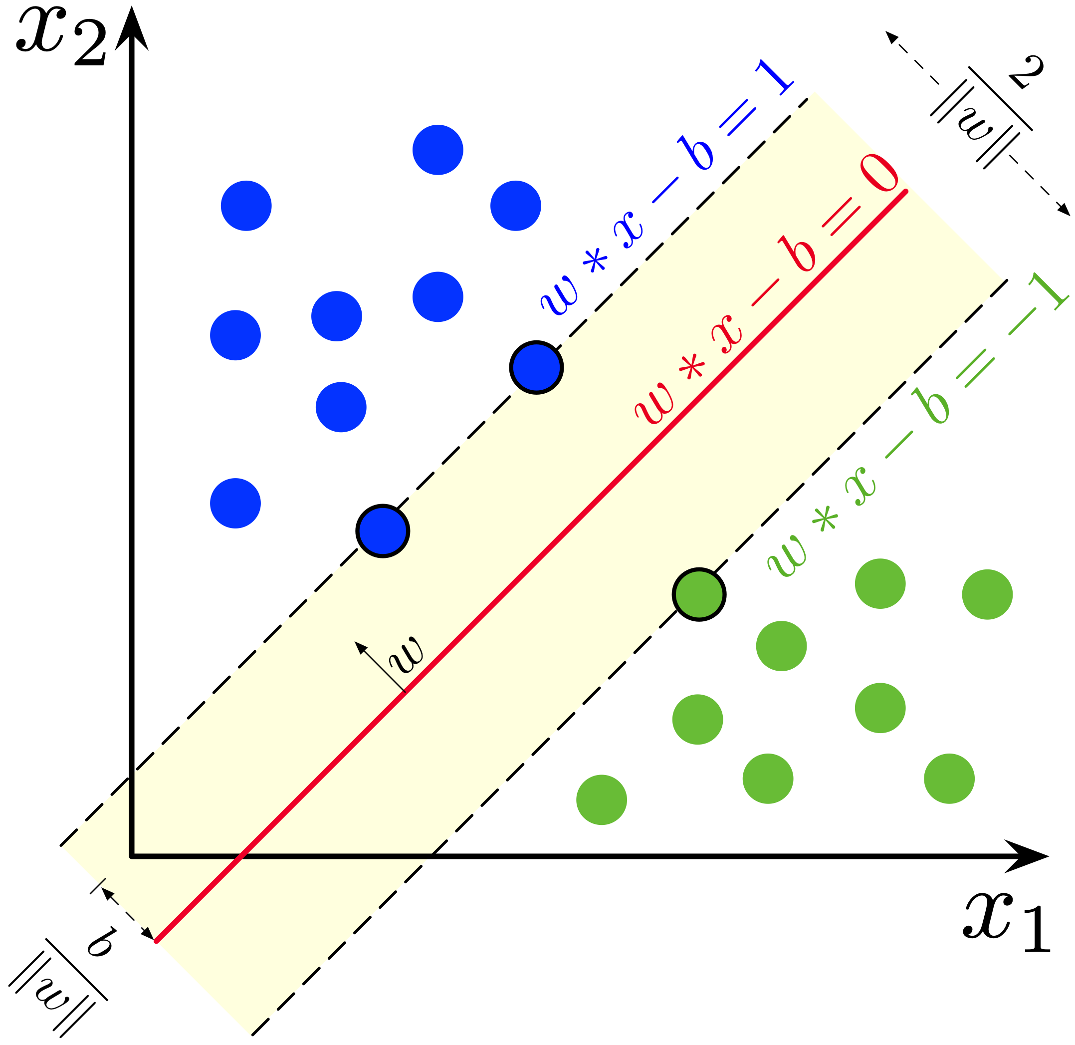
In the diagram above we separate the data with two parallel hyperplanes:

$$w^{\top }x-b=1\text{ (everything on or above belongs to class 1)}$$

and

$$w^{\top }x-b=-1\text{ (everything on or below belongs to class -1)}.$$

Since the distance between these hyperplanes is given by $2/\Vert w\Vert$, we want to minimize $\Vert w\Vert$ in order to maximize the distance. We also have the additional constraints that

$$w^{\top }{x}_i-b\ge 1,\text{ if }{y}_i=1$$

and

$$w^{\top }{x}_i-b\le -1,\text{ if }{y}_i=-1.$$

Multiplying both sides by $y_i$ combines both of these constraints into one. In summary, we get the following optimization problem:

$$\begin{array}{rl}& \underset{w,b}{\mathrm{minimize}}\Vert w{\Vert }_2^2\\ & \text{subject to }{y}_i(w^{\top }{x}_i-b)\ge 1,\forall i\in \{1,\dots ,n\}.\end{array}$$

Once we have solved for $w$ and $b$, we get the classifier function $x\mapsto \text{sgn}(w^{\top }x-b)$.

If the data is not linearly separable, we use soft margins by making use of the hinge-loss function

$$\max (0,1-y_i(w^{\top }{x}_i-b))$$

Then the goal becomes to minimize

$$\Vert w{\Vert }^2+C\left[\frac{1}{n}\sum _{i=1}^n\max (0,1-y_i(w^{\top }x-b))\right]$$

where $C$ is a parameter controlling the trade-off between increased margin size and ensuring the points $x_i$ lie on the correct sides of the margins. As an optimization problem:

$$\begin{array}{rl}& \underset{w,b,\zeta }{\mathrm{minimize}}\Vert w{\Vert }_2^2+C\sum _{i=1}^n{\zeta }_i\\ & \text{subject to }{y}_i(w^{\top }{x}_i-b)\ge 1-{\zeta }_i,{\zeta }_i\ge 0\forall i\in \{1,\dots ,n\}.\end{array}$$

For large enough $C$, this will behave similar to hard margins.

Nonlinear SVM

We can create nonlinear classifiers by applying the “kernel trick” where we replace dot products with kernels. This allows an algorithm to fit the maximum-margin hyperplane to a transformed feature space.

Note that this can increase the generalization error, i.e., how accurately the model can predict outcome data for previously unseen data.

Some common kernels:

• Polynomial (homogeneous): $k(x_i,x_j)=(x_i\cdot x_j{)}^d$
• Polynomial (inhomogeneous): $k(x_i,x_j)=(x_i\cdot x_j+r{)}^d$
• Gaussian radial basis function: $k(x_i,x_j)=\exp (-\gamma \Vert x_i-x_j{\Vert }^2)$ for $\gamma >0$. Often $\gamma =1/(2{\sigma }^2)$
• Sigmoid function: $k(x_i,x_j)=\tanh (\kappa x_i\cdot x_j+c)$ for some $\kappa >0$ and $c<0$

The kernel is related to the transform $\phi (x)$ by the equation $k(x_i,x_j)=\phi (x_i)\cdot \phi (x_j)$. We can represent $w$ in the transformed space by

$$w=\sum _i{\alpha }_i{y}_i\phi (x_i).$$

Thus, for classification functions we can take the dot product with $w$ by using the kernel trick, i.e.,

$$w\cdot \phi (x)=\sum _i{\alpha }_i{y}_{i}k(x_i,x).$$

The Kernel Trick

For nonlinear SVM we mapped our data set into a higher-dimensional space where we could linearly separate. The kernel trick is a method for a learning algorithm to learn a nonlinear function without explicitly mapping into the higher-dimensional space. We want our kernel $k:X\times X\to \mathbb{R}$ which acts in the original space to act as an inner product in the transformed space $Y$. That is, given our transformation $\phi :X\to Y$ our kernel should satisfy

$$k(x,y)=\phi (x)\cdot \phi (y).$$

According Mercer’s theorem, such a function $\phi$ exists if the space $X$ has a suitable measure such that $k$ satisfies

$$\iint g(x)k(x,y)g(y)dxdy\ge 0$$

for all square-integrable functions $g$. If we choose cardinality as our measure, then this condition reduces to

$$\sum _{i=1}^n\sum _{j=1}^{n}k(x_i,x_j)c_i{c}_j\ge 0$$

for all finite sequences of points $(x_1,\dots ,x_n)$ in $X$ and all real-valued coefficients $c_1,\dots ,c_n$.

Recall that the classification vector $w$ in the transformed space is given by

$$w=\sum _{i=1}^n{\alpha }_i{y}_i\phi (x_i).$$

We can obtain the coefficients ${\alpha }_1,\dots ,{\alpha }_n$ by the following optimization problem:

$$\begin{array}{rl}& \text{maximize}f({\alpha }_1,\dots ,{\alpha }_n)=\sum _{i=1}^n{\alpha }_i-\frac{1}{2}\sum _{i=1}^n\sum _{j=1}^n{y}_i{\alpha }_{i}k(x_i,x_j)y_j{\alpha }_j\\ & \text{subject to }\sum _{i=1}^n{\alpha }_i{y}_i=0\text{ and }0\le {\alpha }_i\le \frac{1}{2n\lambda }\text{ for all }i.\end{array}$$

This problem can be solved with quadratic programming. We find an index $i$ such that $0<c_i<1/(2n\lambda )$ and $\phi (x_i)$ lies on the boundary of the margin in the transformed space. Then we solve

$$b=w^{\top }\phi (x_i)-y_i$$

This leaves us with the classifier function

$$x\mapsto \text{sgn}(w^{\top }\phi (x)-b).$$

Scikit-Learn

The python package scikit-learn has support for SVMs. Documentation listing at https://scikit-learn.org/stable/modules/svm.html.

Scikit has three classes for binary and multi-class classifications: SVC, NuSVC, and LinearSVC. All three take in two arrays, $x$ which has shape number of samples-by-number of features and $y$ which is a vector with dimension number of samples.

from sklearn import svm
X = [[0, 0], [1, 1]]
y = [0, 1]
clf = svm.SVC()
clf.fit(X, y)
 
# Predict a new value
clf.predict([[2., 2.]])

The 2d-array $X$ represents the set of points $x_i$ in our data set. Where as, the vector $y$ is the classifications of each point $x_i$. For example, in relation to paragonimiasis, $X$ could have a 2d-vector for each patient (e.g., weight + height) and $y$ would represent if the patient is ELISA positive/negative. Then we could separate that data using SVC.fit.

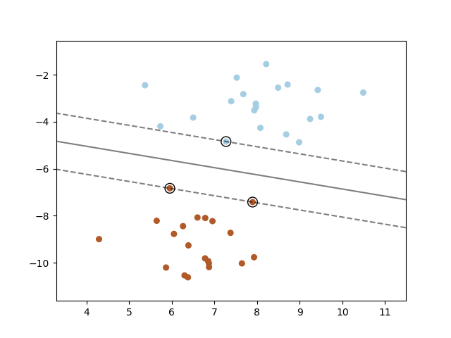
Below is some sample code:

import matplotlib.pyplot as plt
 
from sklearn import svm
from sklearn.datasets import make_blobs
from sklearn.inspection import DecisionBoundaryDisplay
 
# we create 40 separable points
X, y = make_blobs(n_samples=40, centers=2, random_state=6)
 
# fit the model, don't regularize for illustration purposes
clf = svm.SVC(kernel="linear", C=1000)
clf.fit(X, y)
 
plt.scatter(X[:, 0], X[:, 1], c=y, s=30, cmap=plt.cm.Paired)
 
# plot the decision function
ax = plt.gca()
DecisionBoundaryDisplay.from_estimator(
    clf,
    X,
    plot_method="contour",
    colors="k",
    levels=[-1, 0, 1],
    alpha=0.5,
    linestyles=["--", "-", "--"],
    ax=ax,
)
# plot support vectors
ax.scatter(
    clf.support_vectors_[:, 0],
    clf.support_vectors_[:, 1],
    s=100,
    linewidth=1,
    facecolors="none",
    edgecolors="k",
)
plt.show()

which produces the following image: