Parallel Algorithm Design

Notes on chapter 3 of An Introduction to Parallel Computing.

---

Parallelizing an algorithm involves the following:

• Identifying portions that can be performed concurrently
• Mapping concurrent tasks onto multiple processors
• Distributing data to tasks
• Managing data sh2ared by several processors
• Synchronization

Some tasks may need to wait for other tasks to finish executing. This dependency and relative order provides a task-dependency graph, a directed acyclic graph with tasks as nodes and the directed edges indicate dependencies.

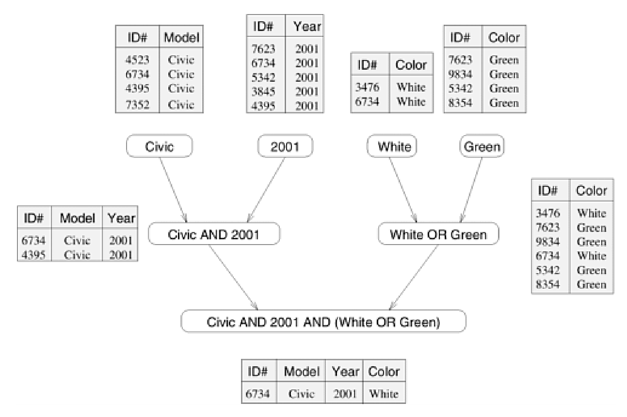
Consider the database query below looking for all 2001 Civics colored either green or white:

MODEL="Civic" AND YEAR="2001" AND (COLOR="Green" OR COLOR="White")

This query can be done by performing a query for each attribute (table for civics, table for 2001, etc.) and taking the intersection or union. Each of these smaller queries can be done concurrently, resulting in the following task-dependency graph:

Note that some processes can be split into smaller tasks in more than one way.

Granularity, Concurrency, and Task-Interaction

The number and size of tasks a problem can be decomposed into determines the granularity of the decomposition. For instance, matrix-vector multiplication $Ax=b$ is fine-grained as we can decompose the problem into single entries of $b$. It can also be coarse-grained by decomposing the problem into larger blocks.

The maximum number of tasks that can be executed simultaneously is called the maximum degree of concurrency. A more useful indicator is the average degree of concurrency. For instance, in our database query above the maximum degree is 4, but the average is $7/3\approx 2.33$. The degree of concurrency is typically proportional to the granularity but also depends on the shape of the task-dependency graph.

In a task-dependency graph, we call the critical path the longest directed path from a start node to a finish node. The sum of weights along the critical path, where the weight is the amount of work, provides a measure of the degree of concurrency. The shorter the critical path, the higher the degree of concurrency.

Increasing the granularity may not always decrease the runtime due to the interaction between tasks. For instance, some tasks may need to wait for other tasks to finish something before accessing any shared memory. The pattern of interaction between tasks can be captured in a graph known as the task-interaction graph.

Processes and Mapping

After decomposing the problem into several tasks, each task must be assigned a computing agent which we call a process. A good mapping should maximize the use of concurrency by mapping independent tasks onto different processes and seek to minimize the runtime by ensuring that processes are available to execute tasks as soon as the become executable.

Decomposition Techniques

There are numerous ways to decompose a problem. The best technique will depend on the problem itself.

Recursive Decomposition

Problems using a divide-and-conquer strategy can often be decomposed using recursion. In divide-and-conquer, a problem is first decomposed into a set of independent subproblems. Each of these subproblems are recursively divided into a smaller set of subproblems. This leads to a natural concurrency approach by solving the subproblems concurrently.

A classic example of this is quicksort. In quicksort a list $A$ of $n$ elements is split into two partitions $A_0\cup A_1$ such that there is some $y\in A$ such that $x<y$ for all $x\in A_0$ and $x\ge y$ for all $x\in A_1$. We then repeat the process for $A_0$ and $A_1$. We can make quicksort concurrent by executing the partitioning of $A_0$ and $A_1$ at the same time. In other words, each subproblem will be split into two tasks that will run concurrently.

Data Decomposition

Another common method for concurrency in algorithms is to partition the data the computation is being performed on.

This can be seen used in something like matrix-matrix multiplication. Assume $A$ and $B$ are $n\times n$ matrices. The product $AB=C$ can be parallalized into four tasks by splitting $A$ and $B$ into four submatrices:

$$\left[\begin{array}{cc}{A}_{11}& A_{12}\\ A_{21}& A_{22}\end{array}\right]\left[\begin{array}{cc}{B}_{11}& B_{12}\\ B_{21}& B_{22}\end{array}\right]=\left[\begin{array}{cc}{A}_{11}{B}_{11}+A_{12}{B}_{21}& A_{11}{B}_{12}+A_{12}{B}_{22}\\ A_{21}{B}_{11}+A_{22}{B}_{21}& A_{21}{B}_{12}+A_{22}{B}_{22}\end{array}\right]$$

From here, each submatrix of $C$ can be solved independently. This is an example of output partitioning.

One may also partition based on input data. Assume we are given a set $T$ containing $n$ transactions and a set $I$ containing $m$ itemsets. Each transaction and itemset contains a small number of items. Suppose we want to find how many times an itemset appears in a transaction. We can decompose this problem based on a partitioning of the input data $T$. For instance, task 1 checks each itemset against transactions $1,\dots ,\lfloor n/2\rfloor$ and task 2 checks each itemset against transactions $\lfloor n/2\rfloor +1,\dots ,n$.

Moreover, we can combine input and output partitioning. For instance, instead of 2 tasks in our transaction problem we can do 4 tasks by splitting each task into 2 subtasks where we only check itemsets $1,\dots ,\lfloor m/2\rfloor$ and itemsets $\lfloor m/2\rfloor +1,\dots ,m$.

When partitioning the input data, there often is a required follow-up computation after all tasks are completed to combine the results together into the final answer.

We could also partition on intermediate data. In our matrix decomposition example, we create four tasks to compute each block of $C$. We can instead create eight tasks by splitting intermediate sum of matrix-products into two additional tasks. In other words, computing

$$\left[\begin{array}{cc}{A}_{11}& A_{12}\\ A_{21}& A_{22}\end{array}\right]\left[\begin{array}{cc}{B}_{11}& B_{12}\\ B_{21}& B_{22}\end{array}\right]=\left[\begin{array}{cc}{A}_{11}{B}_{11}& A_{11}{B}_{12}\\ A_{21}{B}_{11}& A_{21}{B}_{12}\end{array}\right]+\left[\begin{array}{cc}{A}_{12}{B}_{21}& A_{12}{B}_{22}\\ A_{22}{B}_{21}& A_{22}{B}_{22}\end{array}\right]$$

The final sum at the end can be done as a follow-up computation after computing each of the eight matrix-matrix products. Either by doing it as a single process or creating four tasks for each block.

The owner-computes rule states that a partition performs all the computations involving data that it owns.

Exploratory Decomposition

Problems involving the search of a space for a solution can employ exploratory decomposition by partitioning the search space into smaller parts. This differs from data decomposition as when the solution is found other tasks will be killed. Whereas in data decomposition, all tasks are run to completion.

Depending on the solution, an exploratory decomposition may result in less or more work than a serial algorithm.

Speculative Decomposition

Imagine a switch statement in C. One may be able to evaluate one or more of the branches in parallel before we receive the input and know which branch is taken. Once the input is available, we simply use the computation corresponding to the correct branch and all other branches’ computations are discarded.

This speculative approach can result in speedup if the correct branch is slow to determine.