Linear Programming

Linear programming involves solving optimization problems with linear objective functions and linear constraints. The typical LP problem is formed as follows:

$$\begin{array}{rlr}& \underset{\text{x}}{\mathrm{minimize}}& {\text{c}}^{\top }\text{x}\\ & \text{subject to}& {\text{w}}_{LE}^{(i)}\le b_i\text{ for }i\in \{1,2,\dots \}\\ & & {\text{w}}_{GE}^{(j)}\ge b_j\text{ for }j\in \{1,2,\dots \}\\ & & {\text{w}}_{EQ}^{(k)}\le b_k\text{ for }k\in \{1,2,\dots \}\end{array}$$

We typically use matrices to represent linear programs in general form:

$$\begin{array}{rlr}& \underset{x}{\mathrm{minimize}}& c^{\top }x\\ & \text{subject to}& A_{LE}x\le b_{LE}\\ & & A_{GE}x\ge b_{GE}\\ & & A_{EQ}x=b_{EQ}\end{array}$$

We can convert general form linear programs to standard form:

$$\begin{array}{rlr}& \underset{x}{\mathrm{minimize}}& c^{\top }x\\ & \text{subject to}& Ax\le b\\ & & x\ge 0\end{array}$$

We convert $A_{GE}x\ge b_{GE}$ into $-A_{GE}\le -b_{GE}$. We then split $A_{EQ}x=b_{EQ}$ into two constraints: $A_{EQ}x\le b_{EQ}$ and $-A_{EQ}x\le -b_{EQ}$. Next, to ensure all $x$ entries are nonnegative, we replace $x$ with $x^{+}-x^{-}$ and constrain $x^{+}\ge 0$ and $x^{-}\ge 0$ giving us

$$\begin{array}{rlr}& \underset{x^{+},x^{-}}{\mathrm{minimize}}& \left[\begin{array}{c}{c}^{\top }-c^{\top }\end{array}\right]\left[\begin{array}{c}{x}^{+}\\ x^{-}\end{array}\right]\\ & \text{subject to}& \left[\begin{array}{cc}A& -A\end{array}\right]\left[\begin{array}{c}{x}^{+}\\ x^{-}\end{array}\right]\le b\\ & & \left[\begin{array}{c}{x}^{+}\\ x^{-}\end{array}\right]\ge 0\end{array}$$

Each inequality $w^{\top }x\le b$ forms a half-space. The collection of inequalities forms a convex set.

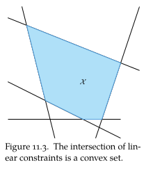
As a result, any local feasible minimum is also a global feasible minimum.

Equality Form

We often represent linear programs in equality form:

$$\begin{array}{rlr}& \underset{x}{\mathrm{minimize}}& c^{\top }x\\ & \text{subject to}& Ax=b\\ & & x\ge 0\end{array}$$

where $x$ and $c$ have $n$ components, $A$ is an $m\times n$ matrix, and $b$ has $m$ components, i.e., there are $n$ nonnegative design variables and a system of $m$ equations.

Any linear program in standard form can be transformed to equality form by changing the constraints:

$$Ax\le b\to Ax+s=b,s\ge 0$$

where $s$ is called a slack variable that enforces equality. For example, consider the following linear program:

$$\begin{array}{rlr}& \underset{x}{\mathrm{minimize}}& 5x_1+4x_2\\ & \text{subject to}& 2x_1+3x_2\le 5\\ & & 4x_1+x_2\le 11\end{array}$$

by introducing two slack variables (one for each constraint) and splitting $x=x^{+}-x^{-}$, we get

$$\begin{array}{rlr}& \underset{x^{+},x^{-},s}{\mathrm{minimize}}& 5(x_1^{+}-x_1^{-})+4(x_2^{+}-x_2^{-})\\ & \text{subject to}& 2(x_1^{+}-x_1^{-})+3(x_2^{+}-x_2^{-})+s_1=5\\ & & 4(x_1^{+}-x_1^{-})+(x_2^{+}-x_2^{-})+s_2=11\\ & & x_1^{+},x_1^{-},x_2^{+},x_2^{-},s_1,s_2\ge 0\end{array}$$

which is in equality form.

Simplex Algorithm

The simplex algorithm is an algorithm for solving linear programs in equality form by moving between vertices of the feasible set. We assume the rows of $A$ are linearly independent and the number of equality constraints is at most the number of design variables $(m\le n)$, i.e., the problem is not over constrained.

Linear programs in equality form have feasible sets that form a convex polytope. Points on the interior of the feasible set are never optimal since we can improve them by moving in the $-c$ direction. Moreover, points on the faces of the polytope can only be optimal if the face is perpendicular to $c$. Finally, vertices have the potential to be optimal.

The simplex algorithm searches over the feasible set’s vertices for the optimal vertex. We can represent every vertex be uniquely defined $n-m$ components of $x$ that equal zero. For example, if $A\in {\mathbb{R}}^{3\times 5}$, then

$$A\left[\begin{array}{c}{x}_1\\ 0\\ x_3\\ x_4\\ 0\end{array}\right]=B\left[\begin{array}{c}{x}_1\\ x_3\\ x_4\end{array}\right]=\left[\begin{array}{c}{b}_1\\ b_2\\ b_3\end{array}\right]$$

uniquely defines a point.

We partition the component indices, $\{1,\dots ,n\}$, into two sets, $\mathcal{B}$ and $\mathcal{V}$, such that

• The design values associated with $\mathcal{V}$ are zero $(i\in \mathcal{V}\Rightarrow x_i=0$)
• The design values associated with $\mathcal{B}$ may be zero ($i\in \mathcal{B}\Rightarrow x_i\ge 0$)
• $\mathcal{B}$ has exactly $m$ elements and $\mathcal{V}$ has exactly $n-m$ elements. We define $x_{\mathcal{B}}$ to be the vector consisting of components of $x$ that are in $\mathcal{B}$, likewise $x_{\mathcal{V}}$ is the vector consisting of components of $x$ that are in $\mathcal{V}$ (note $x_{\mathcal{V}}=0$).

We then find the vertex associated with partition $(\mathcal{B},\mathcal{V})$ by using the $m\times m$ matrix $A_{\mathcal{B}}$ formed by taking the $m$ columns of $A$ selected by $\mathcal{B}$. We then get $x_{\mathcal{B}}=A_{\mathcal{B}}^{-1}b$.

Example: Consider the constraints

$$\left[\begin{array}{cccc}1& 1& 1& 1\\ 0& -1& 2& 3\\ 2& 1& 2& -1\end{array}\right]x=\left[\begin{array}{c}2\\ -1\\ 3\end{array}\right],x\ge 0.$$

We want to verify that $x=[1,1,0,0]$ is feasible and that it has no more than three nonzero component. Notice that

$$A_{1,2,3}=\left[\begin{array}{ccc}1& 1& 1\\ 0& -1& 2\\ 2& 1& 2\end{array}\right]$$

is invertible. Moreover,

$$Ax=A_{1,2,3}{x}_{1,2,3}=A_{1,2,3}{\left[\begin{array}{ccc}1& 1& 0\end{array}\right]}^{\top }=b.$$

Therefore, $x$ is a vertex of the feasible set polytope. Note we could also have used $\mathcal{B}=\{1,2,4\}$.

While every vertex has an associated partition $(\mathcal{B},\mathcal{V})$, not every partition corresponds to a vertex. A partition corresponds to a vertex only if $A_{\mathcal{B}}$ is a nonsingular and $A_{\mathcal{B}}^{-1}b$ is feasible.

The simplex algorithm has two phases:

1. An initialization phase which identifies a vertex partition
2. An optimization phase which transitions between vertex partitions toward a partition corresponding to an optimal vertex.

First-Order Necessary Conditions

Using the Lagrangian for the equality form gives us

$$\mathcal{L}(x,\mu ,\lambda )=c^{\top }x-{\mu }^{\top }x-{\lambda }^{\top }(Ax-b)$$

with the following FONCs:

1. feasibility: $Ax=b$, $x\ge 0$
2. dual feasibility: $\mu \ge 0$
3. complementary slackness: $\mu \odot x=0$ (element-wise product)
4. stationary: $A^{\top }\lambda +\mu =c$

For linear programs, the FONCs are sufficient conditions for optimaility.

We can decompose the stationary condition into $\mathcal{B}$ and $\mathcal{V}$ components:

$$A_{\mathcal{B}}^{\top }\lambda +{\mu }_{\mathcal{B}}=c_{\mathcal{B}}\text{ and }{A}_{\mathcal{V}}^{\top }\lambda +{\mu }_{\mathcal{V}}=c_{\mathcal{V}}.$$

Choosing ${\mu }_{\mathcal{B}}=0$ satisfies the complementary slackness. As a result we get that

$$\lambda ={\left(A_{\mathcal{B}}^{-1}\right)}^{\top }{c}_{\mathcal{B}}.$$

Plugging this in to our $\mathcal{V}$ stationary equation gives us that

$${\mu }_{\mathcal{V}}=c_{\mathcal{V}}-(A_{\mathcal{B}}^{-1}{A}_{\mathcal{V}}{)}^{\top }{c}_{\mathcal{B}}.$$

If ${\mu }_{\mathcal{V}}$ contains negative components, then dual feasibility is not satisfied and the vertex is sub-optimal.

Optimization Phase

At this point of the algorithm we have a partition $(\mathcal{B},\mathcal{V})$ that corresponds to a vertex of the feasible set polytope. We can update the partition by swapping indices between $\mathcal{B}$ and $\mathcal{V}$.

A transition $x\to x^{\prime }$ between vertices must satisfy $A{x}^{\prime }=b$. We choose a entering index $q\in \mathcal{V}$. Then the new vertex $x^{\prime }$ must satisfy

$$A{x}^{\prime }=A_{\mathcal{B}}{x}_{\mathcal{B}}^{\prime }+A_{\{q\}}{x}_q^{\prime }=A_{\mathcal{B}}{x}_{\mathcal{B}}=Ax=b.$$

The index $q$ replaces a leaving index $p\in \mathcal{B}$ and becomes zero in $x_{\mathcal{B}}^{\prime }$. We call such a swap pivoting. We then can solve for the new design point

$$x_{\mathcal{B}}^{\prime }=x_{\mathcal{B}}-A_{\mathcal{B}}^{-1}{A}_{\{q\}}{x}_q^{\prime }.$$

In particular we want when the leaving component is zero, i.e., $(x_{\mathcal{B}}^{\prime }{)}_p=0$. Solving for $x_q^{\prime }$ gives us

$$x_q^{\prime }=\frac{(x_{\mathcal{B}}{)}_p}{(A_{\mathcal{B}}^{-1}{A}_{\{q\}}{)}_p}.$$

We pick the leaving index through the minimum ratio test: select the leaving index $p$ that minimizes $x_q^{\prime }$. With the leaving index selected, we swap $p$ and $q$ between $\mathcal{B}$ and $\mathcal{V}$.

def edge_transition(A, c, b, B, q):
	n = A.shape[1]
	b_inds = sorted(B)
	n_inds = # indices not in B
	AB = A[:,b_inds]
	ABinv = np.linalg.inv(AB)
	d = np.matmul(ABinv, A[:,n_inds[q]])
	xB = np.matmul(ABinv, b)
 
	# Pick the leaving index p that minimizes x'_q
	p, xq = 0, np.inf
	for i in range(d):
		if d[i] > 0:
			v = xB[i] / d[i]
			if v < xq:
				p, xq = i, v
 
	return (p, xq)

Different heuristics can be used to select an entering index $q$:

• Greedy, choose the $q$ that maximally reduces $c^{\top }x$
• Dantzig’s rule, choose $q$ with the most negative entry in $\mu$.
• Bland’s rule, choose the first $q$ with a negative entry in $\mu$.

Example: Consider the equality-form linear program with

$$A=\left[\begin{array}{cccc}1& 1& 1& 0\\ -4& 2& 0& 1\end{array}\right],b=\left[\begin{array}{c}9\\ 2\end{array}\right],c=\left[\begin{array}{c}3\\ -1\\ 0\\ 0\end{array}\right]$$

and the initial vertex defined by $\mathcal{B}=\{3,4\}$. We first extract $x_{\mathcal{B}}$:

$$x_{\mathcal{B}}=A_{\mathcal{B}}^{-1}b={\left[\begin{array}{cc}1& 0\\ 0& 1\end{array}\right]}^{-1}\left[\begin{array}{c}9\\ 2\end{array}\right]=\left[\begin{array}{c}9\\ 2\end{array}\right]$$

and compute $\lambda$:

$$\lambda ={\left(A_{\mathcal{B}}^{-1}\right)}^{\top }{c}_{\mathcal{B}}=0$$

and ${\mu }_{\mathcal{V}}$:

$${\mu }_{\mathcal{V}}=c_{\mathcal{V}}-{\left(A_{\mathcal{B}}^{-1}{A}_{\mathcal{V}}\right)}^{\top }{c}_{\mathcal{B}}=\left[\begin{array}{c}3\\ -1\end{array}\right].$$

Notice that ${\mu }_{\mathcal{V}}$ has a negative element, so $\mathcal{B}$ is sub-optimal. We pivot on the index of the negative element, $q=2$. Using edge transition we get that $p=4$ gives the minimal $x_q^{\prime }$. Thus, we update our set of indices to $\mathcal{B}=\{2,3\}$, ending the first iteration.

Upon the second iteration, we find the indices $\mathcal{B}=\{2,3\}$ is optimal as ${\mu }_{\mathcal{V}}$ has no negative entries.

Initialization Phase

Before performing the optimization phase, we need an initial partition corresponding to a vertex. We can find such a partition by solving an auxiliary linear program:

$$\begin{array}{rlr}& \underset{x,z}{\mathrm{minimize}}& \left[\begin{array}{cc}{0}^{\top }& 1^{\top }\end{array}\right]\left[\begin{array}{c}x\\ z\end{array}\right]\\ & \text{subject to}& \left[\begin{array}{cc}A& Z\end{array}\right]\left[\begin{array}{c}x\\ z\end{array}\right]=b\\ & & \left[\begin{array}{c}x\\ z\end{array}\right]\ge 0\end{array}$$

where $Z$ is the diagonal matrix whose diagonal entries are given by

$$Z_{ii}=\{\begin{array}{ll}+1& \text{if }{b}_i\ge 0\\ -1& \text{otherwise}.\end{array}$$

We solve the auxiliary linear program with a partition that selects only the $z$-values. As a result, the corresponding vertex has $x=0$ and each $z$-element as the absolute value of the corresponding $b$-value.

Example: Consider the following equality-form linear program:

$$\begin{array}{rlr}& \underset{x_1,x_2,x_3}{\mathrm{minimize}}& c_1{x}_1+c_2{x}_2+c_3{x}_3\\ & \text{subject to}& 2x_1-x_2+2x_3=1\\ & & 5x_1+x_2-3x_3=-2\\ & & x_1,x_2,x_3\ge 0\end{array}$$

we can identify a feasible vertex by solving

$$\begin{array}{rlr}& \underset{x_1,x_2,x_3,z_1,z_2}{\mathrm{minimize}}& z_1+z_2\\ & \text{subject to}& 2x_1-x_2+2x_3+z_1=1\\ & & 5x_1+x_2-3x_3-z_2=-2\\ & & x_1,x_2,x_3,z_1,z_2\ge 0\end{array}$$

with an initial vertex defined by $\mathcal{B}=\{4,5\}$. The initial vertex has

$$x_{\mathcal{B}}^{(1)}=A_{\mathcal{B}}^{-1}{b}_{\mathcal{B}}=\left[\begin{array}{c}1\\ 2\end{array}\right]$$

and thus, $x^{(1)}=[0,0,0,1,2]$. From here we can then begin the optimization phase to get the feasible vertex $[0.045,1.713,1.312,0,0]$ in the auxiliary problem, or $[0.045,1.713,1.312]$ in the original problem.