2025-02-28

The Multiscale Flat Norm

For a more detailed look at the flat norm see: Currents and the Flat Norm.

We define an $m$-current to be an element of the dual space of smooth $m$-forms with compact support That is, if ${\Omega }_c^m({\mathbb{R}}^n)$ is the space of smooth $m$-forms with compact support than an $m$-current $T$ is a linear functional

$$T:{\Omega }_c^m({\mathbb{R}}^n)\to \mathbb{R}.$$

One may view an $m$-current as a generalization of oriented subsurfaces. Indeed, given a compact rectifiable oriented set $M$ of dimension $m$, we can construct an $m$-current $R$ given by

$$R(\omega )={\int }_M\omega .$$

If the boundary $\partial M$ is also rectifiable, then it follows by Stokes’ theorem that

$${\int }_{\partial M}\omega ={\int }_{M}d\omega =R(d\omega ).$$

Hence, we define the boundary of an $m$-current $T$ to be the $(m-1)$-current $\partial T$ that satisfies

$$\partial T(\omega )=T(d\omega )$$

for all $m$-forms $\omega$.

Given an $m$-current $T$, we define the mass of $T$ to be given by

$$M(T)=\sup \{T(\omega ):\underset{x}{\sup }\Vert \omega (x)\Vert \le 1\}.$$

As we are viewing currents are oriented surfaces, one may view the mass of a current as it’s $m$-dimensional volume.

Flat Norm

Given an $m$-current $T$, the flat norm is given by

$$\mathbb{F}(T)=\inf \{M(T-\partial S)+M(S):\text{S is a (m+1)-current}\}$$

As an example, consider the figure below:

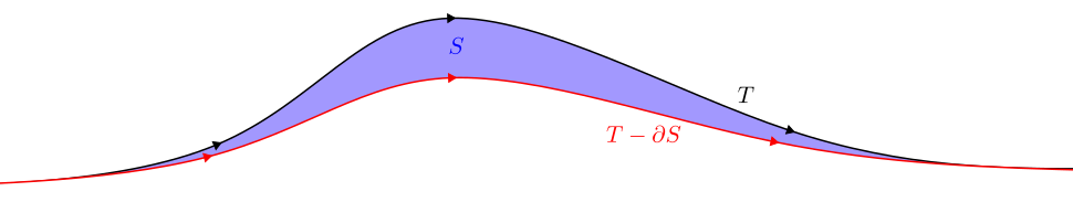
We decompose our 1-current $T$ into a 2-current $S$ and a 1-current $T-\partial S$ such that $M(T-\partial S)+M(S)$ is minimal.

By scaling the affect the mass of $S$ has, we get the multiscale flat norm

Multiscale Flat Norm

Given an $m$-current and $\lambda \ge 0$, the multiscale flat norm is given by

$${\mathbb{F}}_{\lambda }(T)=\inf \{M(T-\partial S)+\lambda M(S):S\text{ is a (m+1)-current}\}.$$

The Median Shape

Given a dataset $x_1,x_2,\dots ,x_n\in \mathbb{R}$, one typically finds the median by sorting the data and picking the middle value. However, one can find the median without sorting:

$$\hat{x}=\underset{x\in \mathbb{R}}{\mathrm{argmin}}\sum _{i=1}^n|x_i-x|.$$

This is known as the geometric median and generalizes to any metric space.

Under the multiscale flat norm, the space of $m$-currents becomes a metric space. Thus, given input $m$-currents $T_1,T_2,\dots ,T_n$, we define the median current to be the $m$-current $\hat{T}$ given by

$$\hat{T}=\underset{T}{\mathrm{argmin}}\sum _{i=1}^n{\mathbb{F}}_{\lambda }(T-T_i).$$

Keeping with our viewing currents as shapes, we get that $\hat{T}$ is the median shape.

One way to generalize this notion is with the mass regularized median shape:

$$\hat{T}=\underset{T}{\mathrm{argmin}}\sum _{i=1}^n{\mathbb{F}}_{\lambda }(T-T_i)+\mu M(T)$$

for some $\mu \ge 0$. In this generalized form, we are applying a penalizing cost given by the mass of the median shape. Thus, we are now looking for the central shape with smallest mass.

Flat Norm on Simplicial Complexes

When it comes to actually computing the median shape, we need to approximate the underlying surface with simplicial complexes. Since a $p$-current $T$ can be viewed as a subsurface of a manifold $M$, we approximate $T$ by a $p$-chain $t$ living in a simplicial complex $K$ that is homotopic to $M$. In this view, our decomposition

$$T=(T-\partial S)+S$$

can be viewed as

$$t=(t-{\partial }_{p+1}s)+s$$

where $t$ is a $p$-chain and $s$ is a $(p+1)$-chain. Thus, we approximate the multiscale flat norm by

$${\mathbb{F}}_{\lambda }(T)\approx \min \{V_p(t-\partial s)+\lambda V_{p+1}(s):s\in C_{p+1}\}$$

where $V_p(t)$ is the $p$-dimensional volume.

Let ${\sigma }_1,\dots ,{\sigma }_m$ and ${\tau }_1,\dots ,{\tau }_n$ be the $p$ and $(p+1)$-simplices of $K$ respectively. Then a $p$-chain $t$ and a $(p+1)$-chain $s$ can be viewed as the sums

$$t=\sum _i{t}_i{\sigma }_i\text{ and }s=\sum _j{s}_j{\tau }_j$$

where $t_i,s_j\in \mathbb{Z}$. Then the multiscale flat norm of a chain $t\in C_p$ is given by

$${\mathbb{F}}_{\lambda }(t)=\underset{x\in C_p,s\in C_{p+1}}{\min }\left\{\sum _{i=1}^m{V}_p({\sigma }_i)|x_i|+\lambda \sum _{j=1}^n{V}_{p+1}({\tau }_j)|s_j|:x=t-{\partial }_{p+1}s\right\}.$$

Median Shape IP

Given a set of $p$-chains $t_1,t_2,\dots ,t_N\in C_p$ we want to find the median chain $\hat{t}$. Using the geometric median as before we get that

$$\hat{t}=\underset{t\in C_p}{\mathrm{argmin}}\sum _{h=1}^N{\mathbb{F}}_{\lambda }(t-t_h).$$

We can solve this problem with an integer program. For each $t-t_h$, denote by $r_h\in C_p$ and $s_h\in C_{p+1}$ the flat norm decomposition, i.e., $t-t_h=r_h+{\partial }_{p+1}s$. Then, denoting the $i$-th component of $r_h$ by $r_{hi}$ gives the following optimization problem:

$$\begin{array}{rlrlr}\text{minimize }& & \sum _{h=1}^N\left(\sum _{i=1}^m{V}_p({\sigma }_i)|r_{hi}|+\lambda \sum _{j=1}^n{V}_{p+1}({\tau }_j)|s_{hj}|\right)& & \\ \text{subject to }& & t-t_h=r_h+{\partial }_{p+1}s& & h=1,2,\dots ,N\\ & & t\in {\mathbb{Z}}^m,r_h\in {\mathbb{Z}}^m,s_h\in {\mathbb{Z}}_m& & h=1,2,\dots ,N\end{array}$$

We want to convert this into an integer program. First notice, that the boundary ${\partial }_{p+1}{s}_h$ can be viewed as a matrix product $B{s}_h$ where $B$ is the $(p+1)$-boundary matrix of $K$. Next, we correct the $|r_{hi}|$ and $|s_{hj}|$ terms by replacing them with

$$r_h=r_h^{+}-r_h^{-}\text{ and }{s}_h=s_h^{+}-s_h^{-}.$$

Thus, our problem becomes

$$\begin{array}{rlrlr}\text{minimize }& & \sum _{h=1}^N\left(\sum _{i=1}^m{V}_p({\sigma }_i)(r_{hi}^{+}+r_{hi}^{-})+\lambda \sum _{j=1}^n{V}_{p+1}({\tau }_j)(s_{hj}^{+}+s_{hj}^{-})\right)& & \\ \text{subject to }& & t-t_h=(r_h^{+}-r_h^{-})+B(s_h^{+}-s_h^{-})& & h=1,2,\dots ,N\\ & & r_h^{+},r_h^{-}\ge 0,s_h^{+},s_h^{-}\ge 0& & h=1,2,\dots ,N\\ & & t\in {\mathbb{Z}}^m,r_h^{+},r_h^{-}\in {\mathbb{Z}}^m,s_h^{+},s_h^{-}\in {\mathbb{Z}}_m& & h=1,2,\dots ,N\end{array}$$

which is now an IP.

Generalized Median Shape IP

To convert our IP into the mass regularized median shape, we need to add the mass of $T$ to our objective function. That is, we add

$$\mu \sum _{i=1}^m{V}_p({\sigma }_i)|t_i|$$

which we can convert to be linear by writing $t=t^{+}-t^{-}$. We also add weights ${\alpha }_1,\dots ,{\alpha }_N\ge 0$ to each input chain where $\sum {\alpha }_h=1$. These changes give the generalized median shape IP:

$$\begin{array}{rlrlr}\text{minimize }& & \mu \sum _{i=1}^m{V}_p({\sigma }_i)(t_i^{+}+t_i^{-})+\sum _{h=1}^N{\alpha }_h\left(\sum _{i=1}^m{V}_p({\sigma }_i)(r_{hi}^{+}+r_{hi}^{-})+\lambda \sum _{j=1}^n{V}_{p+1}({\tau }_j)(s_{hj}^{+}+s_{hj}^{-})\right)& & \\ \text{subject to }& & t^{+}-t^{-}-t_h=(r_h^{+}-r_h^{-})+B(s_h^{+}-s_h^{-})& & h=1,2,\dots ,N\\ & & t^{+},t^{-}\ge 0,r_h^{+},r_h^{-}\ge 0,s_h^{+},s_h^{-}\ge 0& & h=1,2,\dots ,N\\ & & t^{+},t^{-}\in {\mathbb{Z}}^m,r_h^{+},r_h^{-}\in {\mathbb{Z}}^m,s_h^{+},s_h^{-}\in {\mathbb{Z}}_m& & h=1,2,\dots ,N.\end{array}$$

When solving the generalized median shape IP, we solve the relaxed version by dropping the integral requirements.

Total Unimodularity and Integrality

Writing our linear program as a matrix gives the result of

$$\begin{array}{rl}\min & \left[\begin{array}{ccccc}\mu \left[\begin{array}{cc}w& w\end{array}\right]& {\alpha }_1\left[\begin{array}{cccc}w& w& \lambda v& \lambda v\end{array}\right]& {\alpha }_2\left[\begin{array}{cccc}w& w& \lambda v& \lambda v\end{array}\right]& \cdots & {\alpha }_N\left[\begin{array}{cccc}w& w& \lambda v& \lambda v\end{array}\right]\end{array}\right]x\\ \text{s.t.}& \\ & \left[\begin{array}{ccccc}\left[\begin{array}{cc}I& -I\end{array}\right]& \left[\begin{array}{cccc}-I& I& -B& B\end{array}\right]& & & \\ \left[\begin{array}{cc}I& -I\end{array}\right]& & \left[\begin{array}{cccc}-I& I& -B& B\end{array}\right]& & \\ ⋮& & & \ddots & \\ \left[\begin{array}{cc}I& -I\end{array}\right]& & & & \left[\begin{array}{cccc}-I& I& -B& B\end{array}\right]\end{array}\right]x=\left[\begin{array}{c}{t}_1\\ t_2\\ ⋮\\ t_N\end{array}\right]\\ & \\ & \left[\begin{array}{cccccccccccccccc}{t}^{+}& t^{-}& r_1^{+}& r_1^{-}& s_1^{+}& s_1^{-}& r_2^{+}& r_2^{-}& s_2^{+}& s_2^{-}& \cdots & & r_N^{+}& r_N^{-}& s_N^{+}& s_N^{-}\end{array}\right]\ge 0\end{array}$$

where $w=[V_p({\sigma }_i){]}_{i=1}^m$ and $v=[V_{p+1}({\tau }_j){]}_{j=1}^n$.

Totally Unimodular Matrix

A matrix $A$ is totally unimodular (TU) if every square submatrix has determinant 0, 1 or -1.

TU matrices are crucial in integer optimization. Consider the following theorem by Hoffman and Kruskal (1956):

Thm

Let $A\in {\mathbb{Z}}^{m\times n}$. Then the polyhedra $P=\{x\mid Ax\le b,x\ge 0\}$ is integral for all $b\in {\mathbb{Z}}^m$ in which $P\ne \varnothing$ if and only if $A$ is totally unimodular.

Since we are looking for integral solutions, it suffices to show that our matrix $A$ is totally unimodular. Typically one would do this by constructing $A$ with a series of operations that preserve TU. Such operations include, but are not limited to,

• Permuting rows or columns.
• Taking the transpose.
• Multiplying a row or column by -1.
• Adding a row or column of all zeros, or adding a row or column with one nonzero that is $\pm 1$.
• Repeating a row or column.

We can construct our matrix $A$ with the following procedure:

1. Starting with $B$ form $\left[\begin{array}{cccc}-I& I& -B& B\end{array}\right]$.
2. Take the $N$-fold $I$-sum of the matrix $\left[\begin{array}{cccc}-I& I& -B& B\end{array}\right]$.
3. Take the transpose.
4. Copy the first $m$ columns and negate to add a column of $-I$.

While steps 1, 3 and 4 preserve TU, the $N$-fold $I$-sum is not guaranteed to preserve TU. Despite this, all experiments have provided integral solutions.

Open Questions

• Are boundary matrices TU?
• Is $A$ in our linear program TU?
• Solving our LP via the simplex algorithm requires one to check all $2^{4N+2}$ vertices in the worst case scenario. Can we construct a more efficient algorithm that has a polynomial complexity?