Contour Boxplots A Method for Characterizing Uncertainty in Feature Sets from Simulation Ensembles

Authors: Ross Whitaker, Mahsa Mirzargar, and Robert Kirby

Original Paper: https://ieeexplore.ieee.org/document/6634129

---

Introduction

A crucial strategy within uncertainty quantification (UQ) is the construction of ensembles, i.e., collections of different simulations of the same physical process with varying parameters (think weather forecasting). In many cases these simulations provide level sets highlighting a desired feature.

How does one visualize an ensemble of data? One natural strategy is computing various statistics such as mean, variance/covariance, etc. However, these methods do not capture the underlying shape, position and variability of the level sets. The paper seeks to propose a new methodology of shape analysis with the following goals in mind:

• Informative about regions: visualization should apply to contours and convey statistical properties about their shapes, positions, etc.
• Qualitative interpretation: visualizations should provide high-level qualitative interpretations.
• Quantitative interpretation: visualizations should display well-defined statistical content.
• Statistical robustness: aggregate quantities in visualizations should not be sensitive to a small number of examples in the ensemble.
• Aggregation preserving shape: visualizations should display summary information but not hide details.

Band Depth Method and its Generalization to Contours

Order statistics such as median require an ordering on the data. For scalar data, this is easily obtained by simply sorting; however, for non-scalar data this ordering is less clear. One method is data depth, which provides a center-outward ordering of multivariate data. Data depth quantifies how central a particular sample is within a point cloud, with deeper samples considered more representative of the data.

Another method is known as band depth. Given an ensemble of functions $f_i:\mathcal{D}\to \mathcal{R}$, $i=1,2,\dots ,n$, (herein $\mathcal{D}$ and $\mathcal{R}$ are intervals in $\mathbb{R}$) the band depth of each function $f_i$ is the probability that the function lies within the band defined by a random selection of $j$ functions from the distribution. For instance, a function $g(x)$ lies in the band of $j$ randomly selected functions $f_1(x),\dots ,f_j(x)$ if it satisfies the following

$$\begin{array}{r}g(x)\subset B(f_1(x),\dots ,f_j(x))⟺\forall x,\underset{k=1,\dots ,j}{\min }{f}_k(x)\le g(x)\le \underset{k=1,\dots ,j}{\max }{f}_k(x).\end{array}$$

I assume what we are saying here is that the image of $g$ lies in the band of $f_1,\dots ,f_j$ if every point lies between the smallest and largest $f_k$ values. That would match the picture given in Figure 2a. As a set, we can visualize the band $B$ by

$$B(f_1,\dots ,f_j)=\{(x,y)\in \mathcal{D}\times \mathcal{R}\mid \underset{k=1,\dots ,j}{\min }{f}_k(x)\le y\le \underset{k=1,\dots ,j}{\max }{f}_k(x)\}.$$

For a given $j$, we define the band depth as the probability that a function falls into the band formed by an arbitrary set of $j$ other functions chosen at random from the ensemble, i.e.,

$$B{D}^j(g)=\text{Pr}\left[g(\mathcal{D})\subset B(f_1,\dots ,f_j)\right].$$

Band depth is more robust if one takes the sum of all smaller sets to form a band:

$$B{D}_J(g)=\sum _{j=2}^{J}B{D}^j(g).$$

In practice we compute $B{D}^j(g)$ by a sample mean of the indicator function formed by evaluating $BD$ over all appropriately sized subsets from the ensemble (excluding $g$). One should pick subset sizes so that all bands are sufficiently wide to contain $g$ and not too many examples have the same depth. For instance, for $j=3$ an ensemble containing 10 functions should test $C(9,3)=84$ bands to compute $B{D}^j(g)$.

The paper generalizes this notion of band depth and provides a modification that handles small sample sizes and high variability better. Let $E=\{S_1,\dots ,S_n\}$, where $S_i\subset U$ for some universal set $U$, be an ensemble of sets. We say that

$$S\in sB(S_1,\dots ,S_j)⟺\bigcap _{k=1}^j{S}_k\subset S\subset \bigcup _{k=1}^j{S}_k,$$

i.e., a set $S$ is in the band defined by $j$ other sets if it lies between the intersection and unions of the $j$ other sets. For example, consider the figure below:

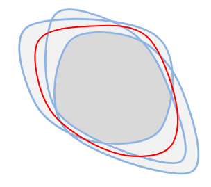
The set $S$ defined by the red contour lies in the contour band of the three blue contours as it lies between the intersection (gray) and the union (light gray).

The band depth is then defined by

$$sB{D}_J(S)=\sum _{j=2}^J\text{Pr}[S\in sB(S_1,\dots ,S_j)].$$

Similar to $BD$, $sB{D}_J$ is computed by taking all appropriately sized subsets of $E$.

The paper outlines an algorithm for applying $sBD$ to a set of level sets by considering the subsets in the plane enclosed by said level sets. Let $F_1(x,y),\dots ,F_n(x,y)$ be a set of fields. For a given $j$, the algorithm for computing the $sBD$ of level sets with value $q$ is

1. Compute the sets (as binary functions on a grid) $S_i=\{(x,y)\mid F_i(x,y)>q\}$ for $i=1,\dots ,n$.
2. For $i=1$ to $n$
   1. Initialize $P_i=0$
   2. For each subset $Q$ of $\{S_1,\dots ,S_n\}$ of size $j$ not containing $S_i$
      1. Compute $S_U={\bigcup }_{S_k\in Q}{S}_k$ and $S_I={\bigcap }_{S_k\in Q}{S}_k$ (can do via min/max operations on the grid)
      2. If $S_I\subset S_i\subset S_U$, then increment $P_i$
   3. Normalize $P_i$ by dividing by the number of subsets $(n-1)$-choose-$r$.
3. Sort the values of $P_i$.

They call this application of set $BD$ to level sets as contour band depth ($cBD$). Note nothing in the above algorithm requires that we work in 2D domains.

This formulation may produce unsatisfactory results if the ensemble is relatively small and the contours vary significantly in shape. Thus, they relax the definition of subset:

$$A{\subset }_{ϵ}B⟺|A|=0\text{ or }\frac{|A-B|}{|A|}<ϵ,$$

i.e., $A$ is the empty set or the percentage of elements $x\in A$ with $x\notin B$ is less than $ϵ$. Under this notion, the epsilon set band is then

$$S\in s{B}_{ϵ}(S_1,\dots ,S_j)⟺\bigcap _{k=1}^j{S}_k{\subset }_{ϵ}S{\subset }_{ϵ}\bigcup _{k=1}^j{S}_k.$$

Methods

The introduction of $sB{D}_{ϵ}$ gives rise to a free parameter $ϵ$. The authors present a method in which $ϵ$ can be tuned automatically to produce the most informative ordering of the data. If there are $m$ sets of $J=2$ against which to compare $n$ contours, then this gives an $m\times n$ matrix $M=[m_{ij}]$ where $m_{ij}$ gives the percentage of mismatch for $S_j\in s{B}_{ϵ}(S_i^1,S_i^2)$ (where $\{S_i^1,S_i^2\}$ is a set of 2 contours from $S_1,\dots ,S_n$) of the worst between union and intersections, i.e.,

$$m_{ij}=\max \left\{\frac{|(S_i^1\cap S_i^2)-S_j|}{|S_i^1\cap S_i^2|},\frac{|S_j-(S_i^1\cup S_i^2)|}{|S_j|}\right\}.$$

If we sum along a column thresholding by $ϵ$ and divide by $m$, we get $cB{D}_{ϵ}$ for that row/sample, i.e., if

$$T_{ϵ}(m_{ij})=\{\begin{array}{ll}{m}_{ij}& \text{if }{m}_{ij}<ϵ,\\ 0& \text{if }{m}_{ij}\ge ϵ\end{array}$$

then the sample mean of the band depth for a particular $ϵ$ is given by

$$\sum _{i=1}^m\frac{1}{m}\sum _{j=1}^n{T}_{ϵ}(m_{ij}).$$

---

Aside:

Recall that given a one-dimensional random variable $X$, a function $f$ is the probability density of $X$ if

$$\text{Pr}[X\in A]={\int }_{A}f(x)\text{d}x.$$

Moreover, $X$ has cumulative distribution $c(x)$ if

$$c(x)=\text{Pr}[X\le x]={\int }_{-\infty }^{x}f(t)\text{d}t.$$

Notice that

$$\begin{array}{rl}\text{Pr}[a<X\le b]& =c(b)-c(a)\\ & ={\int }_{-\infty }^{b}f(x)\text{d}x-{\int }_{-\infty }^{a}f(x)\text{d}x\\ & ={\int }_a^{b}f(x)\text{d}x,\end{array}$$

i.e., by the fundamental theorem of calculus, $c^{\prime }(x)=f(x)$.

TODO: Relearn measure theoretic probability.

---

Assume that a one-dimensional probability density, $p(x)$, has cumulative distribution $c(x)$, i.e., $c^{\prime }(x)=p(x)$. Then (for $J=2$) a particular sample $x$ is in the band of two randomly chosen samples if one sample is less than $x$ and the other sample is greater where the probabilities are given by $c(x)$. That is,

$$???$$

Thus the expected value of the band depth is

$$\begin{array}{rl}{E}_{BD}& ={\int }_{-\infty }^{\infty }xp(x)\text{d}x\\ & {=}^{?}{\int }_{-\infty }^{\infty }(1-c(x))c(x)p(x)\text{d}x\\ & ={\int }_{-\infty }^{\infty }(1-c(x))c(x)c^{\prime }(x)\text{d}x\\ & =\frac{1}{6}.\end{array}$$

As a result, the probability distribution does not matter. Hence we pick the $ϵ$ that satisfies

$$\frac{1}{mn}\sum _{i=1}^n\sum _{j=1}^m{T}_{ϵ}(m_{ij})=\frac{1}{6}.$$