The following is a brief summary of the paper The structure and stability of persistence modules.
Persistence Modules
Persistence Module
Given a poset , a -persistence module is an indexed family of vector spaces (over some field ) with a family of linear maps such that for all and .
We typically visualize persistence modules as a chain of vector spaces:
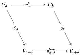
Given two -persistence modules and , we can construct a persistence module homomorphism between and to be a collection of linear maps
such that the linear maps are preserved, i.e., the diagram below commutes for all .
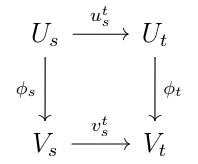
Under such a homomorphism, persistence modules form a category. We denote the homset by .
A particularly useful persistence module is the interval module. Given posets where is an interval, we define the -persistence module with spaces
and maps
For example, if the -interval module is
Interval modules represent features that are present over an interval that are absent elsewhere. For example, in simplicial complex filtrations, the homology groups decompose into a direct sum of interval modules. Each interval module represents a class of cycles that are alive only in the interval .
We can compose two or more persistence modules with the direct sum.
Direct Sum of Persistence Modules
Given two -persistence modules , the direct sum is the -persistence module with spaces
and linear maps
We often do this the opposite direction. Given a persistence module , we want to find interval modules such that
We call such a persistence module decomposable. Note that interval modules are indecomposable because the projection map is either trivial or an isomorphism, i.e., an interval module can only decompose as or .
Gabriel, Auslander, Ringel-Tachikawa, Webb
Let be a persistence module over . Then can be decomposed as a direct sum of interval modules if
- is a finite set; or
- is locally finite and each space is finite-dimensional.
This decomposition is unique up to ordering.
Persistence Diagrams
We often want to visualize the structure of persistence modules. For example, assume we have a persistence module composed of sublevelsets of a function ,
where the maps are given by inclusion when . If we apply the -dimensional singular homology functor, we get a new persistence module of singular homology groups
One may show that each index corresponds to a critical point in the space . So by plotting a point in the extended half-plane if a cycle is born at and dies at , we get what is known as a persistence diagram. For example,
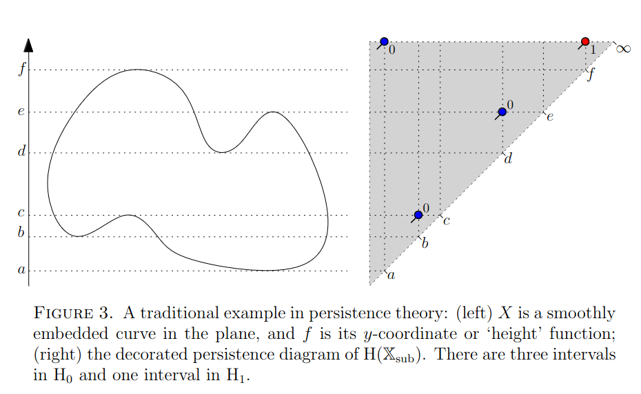
The above figure is an example of a decorated persistence diagram where the points are given a tick direction. In an undecorated persistence diagram the points are not given a tick direction. Note that we have two points at infinity. This implies that there is a 0-cycle born at time that never dies. Likewise there is a 1-cycle born at time that never dies.
Question: What exactly do the tick directions represent?
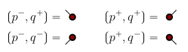
For persistence modules over a poset , it is important to distinguish the topology of the intervals (open, closed, half-open). We do so with decorated real numbers. Given that we have the following four cases:
If the decoration is unknown (or we do not wish to specify), then we use the notation and any of the four options above are possibilities.
Assume that is a decomposable persistence module over , i.e.,
Then we define the decorated persistence diagram of to be the multiset
and the undecorated persistence diagram of to be the multiset
where is the diagonal in the extended half-plane.
Since the decomposition of persistence modules is unique up to order, these definitions are well-defined. In decorated persistence diagrams, the tick direction is drawn depending on the decoration of the interval. The possible tick directions are
Rectangle Measures
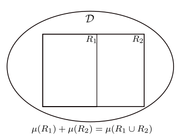
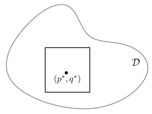
Let . Define
i.e., the set of closed rectangles contained in . A rectangle measure or -measure on is a function such that whenever we get that
In other words, the function is additive with respect to horizontal and vertical splitting.
We define the interior of to be
where is the interior of the rectangle . In other words, the set of points in such that there is an open rectangle contained inside that contains said point.
For decorated points we use the -interior
which behaves the same as the interior but we use the closed rectangle and require the tick to lie inside the rectangle as well.
Equivalence Theorem
Let . There is a bijective correspondence between
- Finite -measures on
- Locally finite multisets in
The measure corresponding to the multiset is related by the formula
where is the multiplicity function, for all rectangles .
Therefore, one may view a finite -measure of a rectangle as simply counting the number of points in that lie inside .
One may extend the equivalence theorem to non-finite -measures by restricting the -interior to only rectangles of finite size
and using horizontal or vertical splitting.
We define the decorated diagram of an -measure to be the unique multiset that satisfies
as described in the equivalence theorem. The undecorated diagram of then ignores the ticks and restricts to the interior, i.e.,
The Persistence Measure
Let be a -persistence module where is a finite subset of , i.e.,
We can represent this module as a quiver
where a filled circle indicates where the module has non-zero rank and the unfilled circle indicate where the module has rank 0. For example if , the six possible interval modules over are
We write
to indicate the number of copies of in the interval decomposition of .
For a persistence module , we define the persistence measure of to be the -measure
for rectangles with . It was shown by Gunnar Carlsson and Vin de Silva that
where . Moreover, if the spaces are finite-dimensional (or at least ), then
where .
For a decomposable persistence module over , one may show that the persistence measure corresponds to the decorated diagram as in the equivalence theorem, i.e.,
Hence, one may say that
Tameness
We say a persistence module is finite if it is a finite direct sum of interval modules. We say it is locally finite if and only if
- each is finite-dimensional
- there is a locally finite set such that is an isomorphism for every pair with .
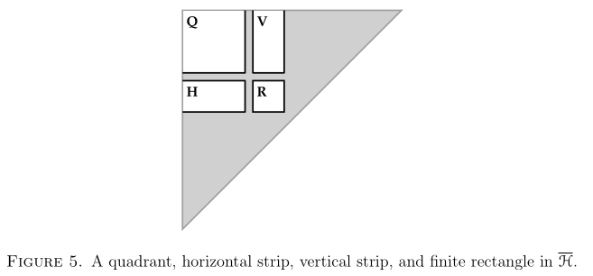
There are four notions of tameness.
- We say is -tame if for every quadrant not touching the diagonal, i.e., for all
- We say is -tame if for every horizontally infinite strip not touching the diagonal, i.e., for all
- We say is -tame if for every vertically infinite strip not touching the diagonal, i.e., for all
- We say that is -tame if for every finite rectangle not touching the diagonal, i.e., for all
The tameness conditions have the following inclusion diagram:
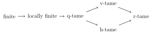
We will be particularly interested in -tame modules.
Interleaving
We say that two persistence modules are isomorphic if there are homomorphisms
such that
That is the diagram
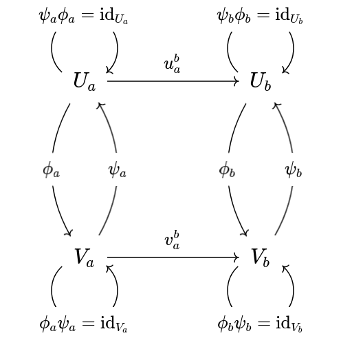
commutes for all indices .
Such a relation in practice is too strong. Instead we use a weaker relation that allows a level of uncertainty. Let be persistence modules over and . A homomorphism of degree is a collection of linear maps
such that the diagram
commutes for all . The set of all homomorphisms of degree between and is denoted by . Note that the composition of a homomorphism of degree and a homomorphism of degree gives a homomorphism of degree .
For the simplest homomorphism of degree is called the shift map, , which is given by the maps
from the underlying persistence diagram structure.
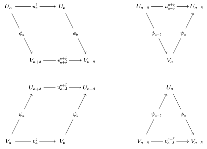
We say that two persistence modules are -interleaved if there are two homomorphisms
such that
In other words, for all the four diagrams below commute:
Given two -interleaved persistence modules, we can continuously interpolate between the two.
Interpolation Lemma
Suppose are a -interleaved pair of persistence modules. Then there exists a 1-parameter family of persistence modules such that are equal to respectively, and are -interleaved.
More specifically, if and are the interleaving maps, then for each in we get a pair of interleaving maps
such that , and
for all . That is, we get a persistence module over .
Let be persistence modules. We define the interleaving distance of and to be
If no such -interleaving exists, we say that .
The interleaving distance forms a pseudometric. It is symmetric and it satisfies the triangle inequality. However, there are non-isomorphic modules with an interleaving distance of zero.
The Bottleneck Distance
The bottleneck distance between two persistence modules is measured using their persistence diagrams. That is, given persistence modules and , the bottleneck distance looks at all possible pairings in and and finds their distance. For unmatched pairs, we take half the distance from the diagonal.
We define a partial matching between multisets and to be a collection of ordered pairs such that
- For every there is at most one such that .
- For every there is at most one such that .
Given a partial matching , we say that it is a -matching if
- If , then
- If is unmatched, then
- If is unmatched, then .
Here we are using the metric on ,
In the case that one or more of the points are at infinity, we use the following distances:
For the unmatched points, we take half the distance down to the diagonal. That is,
The bottleneck distance is then taken to be the smallest possible -matching, i.e., given multisets and ,
Like the interleaving distance, the bottleneck distance satisfies the triangle inequality.
The Isometry Theorem
In the case that and are -tame, the interleaving and bottleneck distances correspond.
Isometry Theorem
If are -tame persistence modules, then
This theorem is the combination of two parts: the stability theorem
and the converse stability theorem