Method
Using an SVM model requires the data to be numerical. While some variables, such as age and height, are numerical, much of the data is categorical in nature. Thus, we require a data preparation preprocess before modeling. We start by converting binary variables into 0s and 1s, e.g., marriage status of the participant is binary; we encode married to 1 and unmarried to 0.
After converting the binary variables, we translate the duration of symptoms. Participants who marked no on the presence of symptom have an empty entry in their corresponding duration symptom. We replace these empty entries with a duration of zero. Next, we convert the duration of symptom from a text entry to a numerical value representing number of days. For example, the duration entry “2 weeks” would be converted into 14.
Some participants marked yes to a symptom but there is no corresponding duration of symptom listed. With the exception of fever, these few participants have been removed from the data set. Fever on the other hand, was missing a duration for approximately 94% of participants. However, over 99% of participants indicated they had a fever. Therefore, we opted to remove the fever related variables.
Once all participants had a duration of symptom (with 0 representing no presence of symptom), the corresponding binary presence of symptom variable become redundant. To speed up on the training process, these variables have been removed.
We perform a similar process with consumption methods. However, the duration and frequency of consumption methods were categorical instead of continuous, e.g., >5 years. Thus, instead of putting a duration of zero for participants who reported to not consume a particular food item, we insert a new category “N/A”.
Like symptoms, once all missing duration and frequency variables have been filled, the binary variables asking if they consume a particular food item become redundant. However, we keep the binary variables for method of consumption. For example, we drop “Consumption_of_fresh_water_crabs” but not “Raw_fresh_water_crabs”.
Finally, we remove any participants who are missing data and one-hot encode the categorical data. One-hot encoding the data turns the categorical variables into several binary variables indicating what category they belong to. For example, the variable for religion turns into two binary variables: one asking if they practice Islam and one asking if they practice Hinduism. Due to the very large variety in the answers, one-hot encoding the village of a participant becomes infeasible. Thus, the village of participants was not taken into account.
The final data set comprises of 9314 participants with 62 variables.
With the now prepared data, we can begin to train an SVM model to classify based on ELISA test result by finding optimal parameters and variables. The training pipeline is laid out as follows:
- The data set is split with 67% of the data used for training and 33% of the data used for testing.
- We perform a 5-fold parameter grid-search to find the set of parameters with the best performing Matthew correlation coefficient (MCC) using all variables.
- With the best found parameters, we perform forward sequential feature selection to find which included variables provide the best MCC by starting with zero variables and adding variables one at a time.
- Finally, we test the best found model on the test set.
Upon training the entire data set, we get a very poorly performing model with an MCC of approximately 0.076. This is likely due to the large imbalance in the various classes as there are only 249 participants with a positive ELISA test result and 9065 participants with a negative ELISA test result.
To accommodate for the imbalance, we train on a subset of the data. We construct a random sample which includes all 249 positive participants and negative participants for various positive integers .
We then perform the same training pipeline as above on the random sample. Once we have found the best performing model, we test the model on another 10 random samples with the same size and positive-to-negative ratio.
Results
We tested on sample sizes with positive-to-negative ratios of 1:1, 1:2, 1:3, 1:4, 1:5 and 1:10. The plot below provides a summary of the results:
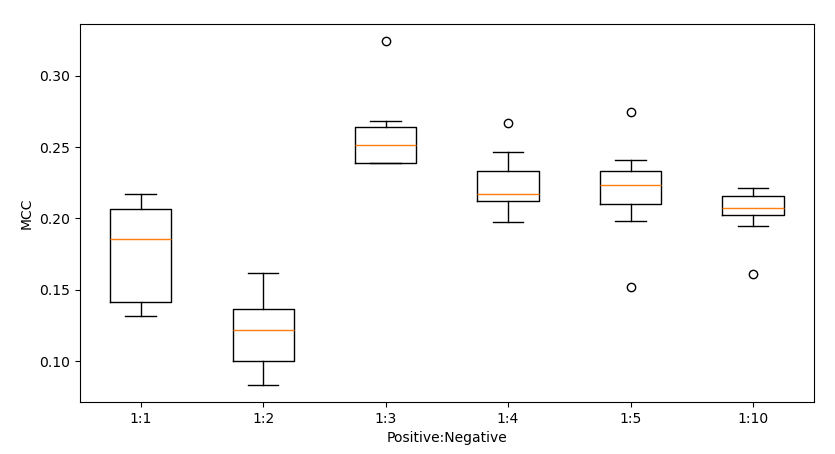
The best performing model was trained with a sample containing 249 positive participants and 747 negative participants (1:3 ratio) with an average MCC of 0.257 and average accuracy of 77.37%. The model used a degree 3 RBF kernel with and class weights of 1:2. The selected variables where:
- Age_of_the_study_participant
- Marital_status_of_the_participant
- Height_of_the_study_participant_in_Cms
- Weight_of_the_study_participant_in_Kgs
- Other_symptoms
- Have_you_taken_any_treatment_or_actions
- Have_you_ever_been_treated_for_TB
- Raw_fresh_water_crabs
- Roasted_fresh_water_crabs
- Smoked_fresh_water_crabs
- Soup_fresh_water_crabs
- Cooked_fresh_water_crabs
- Soup_cray_fish
- Cooked_wild_boar_meat
- Duration_of_cough
- Duration_of_expectoration
- Duration_of_chest_pain
- Duration_of_loss_of_appetite
- Duration_of_blood_in_sputum
- Duration_of_night_sweats
- Duration_of_weight_loss
- Duration_of_shortness_of_breath
- Duration_of_tiredness
- Sex_of_the_study_participant_Female
- Sex_of_the_study_participant_Male
- Sex_of_the_study_participant_Transgender
- Religion_of_the_participant_Hindu
- Religion_of_the_participant_Islam
- Educational_qualification_of_the_study_participant_Graduate/Degree/Diploma
- Educational_qualification_of_the_study_participant_Illiterate
- Educational_qualification_of_the_study_participant_Post-graduate