Bi-Filtration and Stability of TDA Mapper for Point Cloud Data

Authors: Wako Bungula and Isabel Darcy

Full paper can be found at https://arxiv.org/abs/2409.17360.

---

Given a topological space $X$ equipped with a continuous function $f:X\to \mathbb{R}$, a filtration of covers of $\mathbb{R}$ gives rise to a filtration of covers of $X$, which in turn gives rise to a filtration of the Mapper graphs. This filtration of Mapper graphs induces a filtration of homology groups. This paper is instead interested in point cloud data.

Filtrations via Nerves of a Cover

Def

Given a family of covers, $\mathbb{U}=\{{\mathbb{U}}_{\lambda }\}$ equipped with a family of maps $\{u^{{\lambda }_i,{\lambda }^j}:{\mathbb{U}}_{{\lambda }_i}\to {\mathbb{U}}_{{\lambda }_j}\mid \forall {\lambda }_i\le {\lambda }_j\}$ for some parameter $\lambda$ where if $u^{{\lambda }_i,{\lambda }_j}(U)=V$ then $U\subseteq V$, we say there is a filtration of covers if $u^{{\lambda }_j,{\lambda }_k}\circ u^{{\lambda }_i,{\lambda }^j}=u^{{\lambda }_i,{\lambda }_k}$.

Let $X$ be a topological space with $N$ coverings, $\{{\mathbb{U}}^i{\}}_{i=1}^N=\{\{U_{\alpha }^i{\}}_{\alpha \in A_i}{\}}_{i=1}^n$ and $h$ is the family of functions

$$\cdots \to A_i\stackrel{h^{i,j}}{\to }{A}_j\stackrel{h^{j,k}}{\to }{A}_k\to \cdots$$

where $i\le j\le k$ and for $\alpha \in A_i$, $h^{i,j}(\alpha )=\beta$ implies that $U_{\alpha }^i\subseteq U_{\beta }^j$ and $h^{j,k}\circ h^{i,j}=h^{i,k}$. Then $h$ induces a filtration of simplicial maps

$$\cdots \to \text{Nrv}({\mathbb{U}}^i)\stackrel{\text{Nrv}(h^{i,j})}{\to }\text{Nrv}({\mathbb{U}}^j)\stackrel{\text{Nrv}(h^{j,k})}{\to }\text{Nrv}({\mathbb{U}}^k)\to \cdots$$

where $\text{Nrv}(h^{i,j})$ is a simplicial map defined on the vertex set of $\text{Nrv}({\mathbb{U}}^i)$ such that if $[v_0,v_1,\dots ,v_n]\in \text{Nrv}({\mathbb{U}}^i)$ then $[\text{Nrv}(h^{i,j})(v_0),\dots ,\text{Nrv}(h^{i,j})(v_n)]\in \text{Nrv}({\mathbb{U}}^j)$ where $\text{Nrv}(h^{i,j})(v_k)=v_{h^{i,j}(k)}$.

Theorem 1

A filtration of covers induces a well-defined filtration of simplicial complexes.

Theorem 2

A filtration of simplicial complexes induces a filtration of homology groups.

Filtration of Mapper Graphs

The traditional Mapper depends on several parameters such as bin size and percent overlap. Recall that in the Mapper we make use of a filter function $f:X\to Z$ and form a cover of $Z$ that is then pulled back by $f$ to create a cover of $X$. Then each pullback cover is clustered to form the cluster cover.

While a filtration of covers of $Z$ induces a filtration of pullback covers of $X$, it is not clear that it induces a filtration of cluster covers. The paper claims there are instances in which we do not get a filtration of cluster covers. Clearly a filtration of cluster covers induces a filtration of their nerves and hence their homology groups. Thus, we simply only need to check when a filtration of covers induces a filtration of cluster covers.

Remark: This is all for the filtration as defined above (i.e., the Multiscale mapper). We can still construct a filtration starting with the cluster covers (see Steinhaus Filtration and Stable Paths in the Mapper).

No Filtration of Cluster Covers: Complete/Average-Linkage, bin size.

Two common clustering algorithms used in Mapper is single-linkage and DBSCAN as they provide the correct connected components of a dataset. But, two points far from each other may be put in the same cover if there is a chain of points connecting them.

The authors construct an example in which the Mapper parameterized by bin size fails to produce a filtration. More specifically, they take a data set $X\subset \mathbb{R}$ and the filter function $f(x)=x$ and construct two covers of $f(X)$:

1. Two interval $I_1$ and $I_2$ with 20% overlap
2. Two intervals $J_1$ and $J_2$ with 50% overlap Note that $f^{-1}(I_1)\subseteq f^{-1}(J_1)$ and $f^{-1}(I_2)\subseteq f^{-1}(J_2)$.

This forms a simple filtration on the dataset $X$

$$\{f^{-1}(I_1),f^{-1}(I_2)\}\to \{f^{-1}(J_1),f^{-1}(J_2)\}.$$

They then used single-linkage clustering on the cover. After clustering, there is a cover that lies in $f^{-1}(I_2)$ but is not contained any clusters of $f^{-1}(J_2)$. In other words, a filtration on the pullback cover parameterized by bin size failed to induce a filtration on the cluster cover.

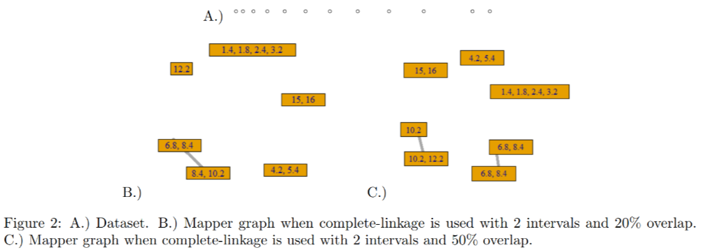
Notice that the cover $\{8.4,10.2\}$ in the Mapper graph corresponding to $I_1,I_2$ (B) is lost in the Mapper graph corresponding to $J_1,J_2$ (C).

DBSCAN

The general idea of DBSCAN is to cluster a set of dense points together, and if there is a set of low-density points they are considered noise. DBSCAN is configured by two parameters: $MinPts\in \mathbb{Z}$ and radius $ϵ\in \mathbb{R}$. An $ϵ$-neighborhood of a point $p$ is considered a dense set if the neighborhood contains at least $MinPts$ points, i.e.,

$$|N_{ϵ}(p)|=|\{q\in X\mid d(p,q)\le ϵ\}|\ge MinPts.$$

KeplerMapper defaults to $ϵ=0.5$ and $MinPts=3$.

• A point $p$ is a core point if $|N_{ϵ}(p)|\ge MinPts$
• A point $q$ is a border point if $|N_{ϵ}(q)|<MinPts$ and there is a core point $p$ such that $q\in N_{ϵ}(p)$.
• A point $r$ is noise if $r$ is neither a core point nor a border point.

Def

A point $q$ is directly density-reachable from a point $p$ w.r.t. $ϵ$ and $MinPts$ if $p$ is a core point and $q\in N_{ϵ}(p)$.

Def

A point $q$ is density-reachable from a point $p$ w.r.t. $ϵ$ and $MinPts$ if there is a sequence of points $p={\alpha }_1,{\alpha }_2,\dots ,{\alpha }_n=q$ such that ${\alpha }_{i+1}$ is directly density-reachable from ${\alpha }_i$.

Def

A point $p$ is density-connected to a point $q$ w.r.t. $ϵ$ and $MinPts$ if there is a point $o$ such that both $p$ and $q$ are density reachable from $o$ w.r.t. $ϵ$ and $MinPts$.

Question: Why the distinction between density-reachable and density-connected? It seems like $q$ being density-reachable from $p$ implies that $p$ and $q$ are density-connected.

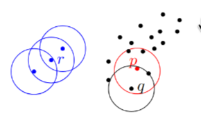
Answer: Density-reachable is not a symmetric relation. For example, in the dataset below

the point $s$ is (directly) density-reachable to the points $p$ and $q$, but $p$ and $q$ are not density-reachable to $s$ because $s$ is not a core point ($|N_{ϵ}(s)|<MinPts$). But $p$ is density-connected to $s$ because there is a point $o=p$ such that $p$ and $s$ are density-reachable from $o$.

Def

Let a dataset $X=C_1\bigsqcup C_2\bigsqcup \cdots \bigsqcup C_n\bigsqcup N$ where $N$ is a set of noise points and $C_i$ is a cluster w.r.t. $ϵ$ and $MinPts$ satisfying:

• (Maximality) $\forall p,q$, if $p\in C_i$, $q\notin {\bigcup }_{j=1}^{i-1}{C}_j$, and $q$ is density-reachable from $p$ w.r.t. $ϵ$ and $MinPts$, then $q\in C_i$.
• (Connectivity) $\forall p,q\in C_i$, $p$ is density-connected to $q$ w.r.t. $ϵ$ and $MinPts$.

In summary, a DBSCAN cluster of a dataset $X$ is a set of points $C_i$ such that any two points $p,q\in C_i$ are density-connected and there is no larger such cover $C_i$.

The paper constructs an example in which the assignment of a point is dependent on the order the data is listed.

Def

A point $s$ is a free-border point w.r.t. $ϵ$ and $MinPts$ if there exists two points $p$ and $q$ such that

• $s\in N_{ϵ}(p)$ and $|N_{ϵ}(p)|\ge MinPts$
• $s\in N_{ϵ}(q)$ and $|N_{ϵ}(q)|\ge MinPts$
• $|N_{ϵ}(s)|<MinPts$, and
• $p$ is not density connected to $q$.

For the example, the dataset given below:

contains a free-border point $s$ when $ϵ=d(p,s)=d(s,q)$ and $MinPts=5$.

The paper claims that as long as there are no free-border points a filtration of covers of $X$ gives a filtration of cluster covers of $X$ as bin size increases, the $ϵ$ parameter increases, or $MinPts$ decreases.

Lemma 2

Let $X$ be a dataset.

• If $p$ is a core point, then there is a cluster $C$ containing $p$ and if $q\in C$ then $q$ is density-reachable from $p$.
• Let $C$ be a cluster. Then there is a point $p\in C$ that is a core point. If $q\in C$ then $q$ is density-reachable from $p$.

In other words, the Lemma above states that a cluster is determined by any of its core points and the core points do not change depending on the order of the dataset.

Filtration of cluster covers: DBSCAN, bin size.

Free-border points can results in a failure to filter the cluster covers. Consider the example below:

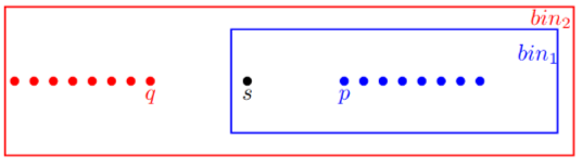
Assume that $q$ is ordered before $s$ and $p$, $MinPts=5$ and $ϵ=d(p,s)=d(q,s)$. When DBSCAN is applied to $bi{n}_1$ a cluster $C_p^{bi{n}_1}$ is formed w.r.t. $ϵ$ and $MinPts$ containing $s,p$ and all points to the right of $p$. When we apply DBSCAN to $bi{n}_2$ we get two clusters w.r.t. $ϵ$ and $MinPts$: $C_q^{bi{n}_2}$ contaning points $s$, $q$ and points to the left of $q$ and $C_p^{bi{n}_2}$ containing $p$ and points to the right of $p$.

This is an issue as $bi{n}_1\subset bi{n}_2$ but $C_p^{bi{n}_1}⊈C_p^{bi{n}_2}$. Thus, the free-border point $s$ results in a filtration of cluster covers parameterized by bin size being invalid.

The critical point here is the free-border point $s$. In the absence of free-border points the issue disappears:

Lemma 4

Suppose there are no free-border points when DBSCAN is used to cluster. If $bin1\subseteq bin2$., then $C_p^{bin1}\subseteq C_p^{bin2}$.

Therefore, if there are no free-border points than there is a filtration of cluster covers parameterized by bin size. As a corollary, if $MinPts\in \{1,2\}$ then there is a filtration of cluster covers parameterized by bin size as there will be no free-border poitns.

Filtration of cluster covers: DBSCAN, ϵ

Notice that if ${ϵ}_0\le {ϵ}_1$ then if $p$ is a core point w.r.t ${ϵ}_0$ then $p$ is a core point w.r.t. ${ϵ}_1$. Thus, one could potentially construct a filtration parameterized by $ϵ$.

Lemma 5

Suppose $X$ is a data set, ${ϵ}_0\le {ϵ}_1$, and $MinPts$ and $\mathbb{B}=\{bi{n}_i\}$ are fixed. If there are no free-border points w.r.t. ${ϵ}_1$ and $MinPts$ then $C_p^{{ϵ}_0}\subseteq C_p^{{ϵ}_1}$.

Therefore, the absence of free-border points indicates that there is a filtration of cluster covers parameterized by $ϵ$.

Filtration of cluster covers: DBSCAN, MinPts

Notice that if $MinPt{s}_0\ge MinPt{s}_1$ and $p$ is a core point w.r.t. $ϵ$ and $MinPt{s}_0$, then $p$ is also a core point w.r.t. $ϵ$ and $MinPt{s}_1$.

Lemma 6

Suppose $X$ is a dataset, $MinPt{s}_0\ge MinPt{s}_1$, and $ϵ$ and $\mathbb{B}$ are fixed. If there are no free-border points w.r.t. $ϵ$ and $MinPt{s}_1$ then $C_p^{MinPt{s}_0}\subseteq C_p^{MinPt{s}_1}$.

Therefore, the absence of free-border points indicates that there is a filtration of cluster covers parameterized by decreasing $MinPts$.

Filtration of Simplicial Complexes and Homology Groups

If there are no free-border points, then we can construct simplicial and homological filtrations parameterized by

• Bin size
• $ϵ$
• $MinPts$

Bi-Filtrations and Stability

The paper claims that DBSCAN is not stable under small perturbation. Let $X$ be a dataset and $X_{\delta }$ the dataset obtained by perturbing $X$ by at most $\delta$, i.e., there is some function $\Delta :X\to X_{\delta }$ such that $d(x,\Delta (x))\le \delta$ for all $x\in X$. We say that

$$d(X,X_{\delta })=\max \{\min \{d(x,y)\mid x\in X,y\in X_{\delta }\}\}\le \delta .$$

How does applying DBSCAN to $X$ and $X_{\delta }$ vary?

For example, consider the following two datasets:

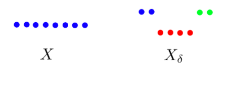
If we let $ϵ$ be the distance between two points in $X$ and $MinPts=2$, then $X$ is clustered into a single set where as $X_{\delta }$ is clustered into three disjoint sets.

We construct a two-dimensional filtration (bi-filtration) parameterized by $ϵ$ and bins $\mathbb{B}$, leaving $MinPts$ fixed. Note that each parameter alone gives a filtration (assuming no free-border points), that is, given a dataset $X$ there is a filtration of cluster covers

$$\{c^{{\mathbb{B}}_i,{\mathbb{B}}_j}:{\mathbb{C}}_{{\mathbb{B}}_i}\to {\mathbb{C}}_{{\mathbb{B}}_j}\mid \forall {\mathbb{B}}_i\le {\mathbb{B}}_j\}$$

which induces a filtration of simplicial complexes

$$\{{\Phi }^{{\mathbb{B}}_i,{\mathbb{B}}_j}:\text{Nrv}({\mathbb{C}}_{{\mathbb{B}}_i})\to \text{Nrv}({\mathbb{C}}_{{\mathbb{B}}_j})\mid \forall {\mathbb{B}}_i\le {\mathbb{B}}_j\}$$

which induces a filtration of $k$-th homology groups

$$\{f^{{\mathbb{B}}_i,{\mathbb{B}}_j}:H_k(\text{Nrv}({\mathbb{C}}_{{\mathbb{B}}_i}))\to H_k(\text{Nrv}({\mathbb{C}}_{{\mathbb{B}}_j}))\mid \forall {\mathbb{B}}_i\le {\mathbb{B}}_j\}.$$

A similar set of filtrations exist parameterized by $ϵ$. Combining the two together gives a set of bi-filtrations where $\mathbb{B}$ is one dimension and $ϵ$ is the other.

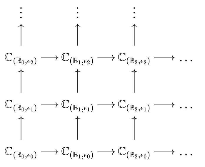
We can perform the same with $X_{\delta }$ to get another set of bi-filtrations ${\mathbb{D}}_{({\mathbb{B}}_i,{ϵ}_j)}$.

Interleaving of Bi-filtrations

See The structure and stability of persistence modules for more details.

Def

Let $P_n$ be a polynomial ring in $n$ variables $x=\{x_1,x_2,\dots ,x_n\}$. An $n$-graded module is a $P_n$ module $M$ such that $M\cong {⨁}_{a\in {\mathbb{R}}^n}{M}_a$ and $x^b(M_a)\subset M_{a+b}$ for all $a\in {\mathbb{R}}^n$, $b\in [0,\infty {)}^n$ where $M_a$ is a vector space over some field $k$. The action of $x^{b-a}$ gives rise to a linear map $\phi :M_a\to M_b$ for all $a\le b\in {\mathbb{R}}^n$.

This is unnecessarily complicated. We’re just taking persistence modules parameterized by two variables. Thus, we have a set of vector spaces $M_{(x,y)}$ and a set of linear maps $\phi :M_{(x,y)}\to M_{(x^{\prime },y^{\prime })}$ for all $(x,y)\le (x^{\prime },y^{\prime })$.

Def

For $M$ an $n$-graded module and $v\in {\mathbb{R}}^n$, $M(v)$ is the shifted module such that $M(v{)}_u=M_{v+u}$.

Def

For $M$ and $n$-graded module, $\overline{\xi }=\{\xi ,\xi ,\dots ,\xi \}\in {\mathbb{R}}_{+}^n$ and $M(\overline{\xi })$,

$${\phi }_M^{\overline{\xi }}:M\to M(\overline{\xi })$$

is the (diagonal) $\xi$-transition morphism such that ${\phi }_M^{\overline{\xi }}(M_a)={\phi }_M(a+\overline{\xi })$.

This is just $ϵ$-homomorphisms but now $ϵ\in {\mathbb{R}}^n$.

Def

Let $\xi \ge 0$. Two $n$-modules $M$ and $N$ are $\xi$-interleavd if there are morphisms $f:M\to N(\xi )$ and $g:N\to M(\xi )$ such that ${\phi }_N^{2\xi }=f(\xi )\circ g$ and ${\phi }_M^{2\xi }=g(\xi )\circ f$.

Again, this is just $ϵ$-interleaving but now $ϵ\in {\mathbb{R}}^n$.

Stability Against Perturbation

Assume there are no free-border points. Then as described above we get a filtration for $X$

$$\mathcal{C}:\cdots \to {\mathbb{C}}_{({\mathbb{B}}_i,{ϵ}_j)}\to {\mathbb{C}}_{({\mathbb{B}}_k,{ϵ}_{\ell })}\to \cdots$$

and a filtration for $X_{\delta }$

$$\mathcal{D}:\cdots \to {\mathbb{D}}_{({\mathbb{B}}_i,{ϵ}_j)}\to {\mathbb{D}}_{({\mathbb{B}}_k,{ϵ}_{\ell })}\to \cdots .$$

According to proposition 1, there are family of maps $\varphi$ and $\psi$ such that the diagram below commutes:

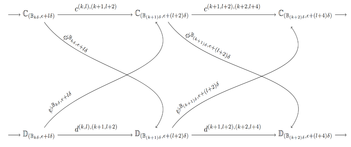
In other words, the filtrations $\mathcal{C}$ and $\mathcal{D}$ are $2\delta$-interleaved. This $2\delta$-interleaving induces a $2\delta$-interleaving between their homologies $H_k(\mathcal{C})$ and $H_k(\mathcal{D})$.