Box Filtration

Questions:

• Unsure how the weights $w_x$ for a point $x\in N$ are determined
• How to solve the LP for box expansion?
• What if a point $x\in X$ lies on the boundary of two or more pixels?

Full paper can be found at: https://arxiv.org/abs/2404.05859v2

Notation used:

Notation	Definition/Explanation
$\sigma$	unit pixel
$m_{\sigma },w_{\sigma },\theta (\sigma )$	centroid, weight, and number of points in pixel $\sigma$
$w_x$	weight of point $x$
$\alpha ,\pi$	$\alpha \in [0,1],\pi \in {\mathbb{R}}_{+}$ are parameters for linear optimization
$\mathcal{U}(0)$	initial collection of boxes that covers $X$
$V$	$V=[l_1,u_1]\times \cdots \times [l_n,u_n]$ is a box in $\mathcal{U}(0)$.
$V[j\pi ]$	$j$-th expansion of $V$
$B(V,\pi )$	$\pi$-neighborhood box of $V$: $(l_1-\pi ,u_1+\pi )\times \cdots \times (l_n-\pi ,u_n+\pi )$
$C_{\alpha }(V,N)$	cost of $V$ in the neighborhood $N\supset V$
${\text{Sol}}_{\alpha }(V,N)$	set of optimal solutions for input box $V$ and neighborhood $N\supset V$
$\mathcal{U}(j\pi )$	$j$-th cover $\forall V\in \mathcal{U}(0)$
$\Theta (V)$	set of pixels with $m_{\sigma }\in V$, $\theta (\sigma )\ne 0$
${\psi }_1(V),{\psi }_2(V),{\psi }_3(V)$	rounded boxes for given box $V$
$K(\mathcal{U})$	filtration corresponding to cover $\mathcal{U}$

Introduction

There are many newly proposed approaches to solve the outlier problem, such as, a distance to measure class of filtration which uses density functions and kernel density estimates to grow the balls guided by where the measure is greater; as a result ignoring isolated outliers. Another proposed approach is a bi-filtration where both distance and density thresholds are treated as parameters. All of these approaches center on using balls centered around points to control the filtration. Since balls grow uniformly, a symmetry bias may occur.

Building filtrations by growing hyper-rectangles (boxes) non-uniformly in different directions based on the distribution of points may be a better approach to capturing the data’s topological features. Since boxes are still convex, the nerve lemma still applies, i.e., the simplicial complex defined as the nerve of the boxes has the same homotopy type as the collection.

The paper defines a new framework called the box filtration of a point-cloud data (PCD) $X\in {\mathbb{R}}^n$ built by growing boxes as the convex sets covering $X$. Two approaches to handle boxes are provided: a point cover where each point is assigned a box at start, and a pixel cover that “works with a pixelization of the space of the PCD”. A filtration is built by expanded the boxes in a manner that minimizes an objective function. An expansion algorithm is provided.

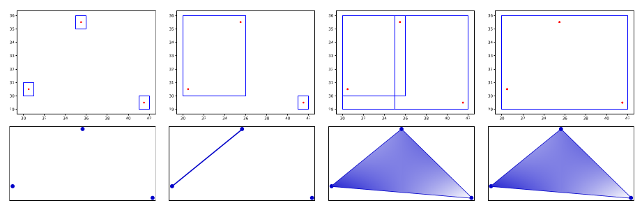
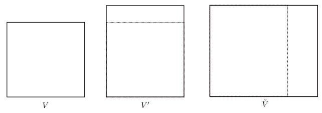
The box filtration can produce results that are more resilient to noise and with less symmetry bias than VR and distance-to-measure (DTM) filtrations. Any box cover of $X$ also gives a mapper, hence the box filtration can function as a mapper framework. For example, the top row above is the point cloud ($X$) and the box covers. The bottom row is the nerve of each.

Construction

Definition 2.1 (Box)

A box in ${\mathbb{R}}^n$ is defined as the $n$-fold Cartesian product $[l_1,u_1]\times \cdots \times [l_n,u_n]$ where $l_i\le u_i$, $\forall i\in \{1,\dots ,n\}$.

Note that a boxes dimension may be lower than $n$ if $l_i=u_i$ for some $i\in \{1,\dots ,n\}$.

Point Cover

Given a finite PCD $X\in {\mathbb{R}}^n$, the initial cover $\mathcal{U}(0)$ of its point cover consists of a collection of hypercubes (${\ell }_{\infty }$-balls) or boxes such that each point is located in a single box. A box may contain more than one point. Every box $V\in \mathcal{U}(0)$ is called a pivot box. We want to expand each pivot box using two parameters $\pi \in {\mathbb{R}}_{+}$ and $\alpha \in [0,1]$ using linear optimization where $\pi$ represents a step size to expand the boxes by and $\alpha$ controls the relative weight in the objective function. The set of optimal solutions for an input box $V$ and neighborhood $N=B(V,\pi )=(l_1-\pi ,u_1+\pi )\times \cdots \times (l_n-\pi ,u_n+\pi )$ is denoted ${\text{Sol}}_{\alpha }(V,N)$.

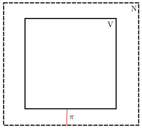
Let $\tilde{V}=[\widetilde{l_1},\widetilde{u_1}]\times \cdots \times [\widetilde{l_n},\widetilde{u_n}]\supseteq V$ be an expanded box in the neighborhood $N$. The objective function of the linear program is denoted by $C_{\alpha }(\tilde{V},N)$. The goal is to cover all points, the points in $N$ that are not covered by $\tilde{V}$ result in a cost in $C_{\alpha }(\tilde{V},N)$. The farther away a non-covered point is from $\tilde{V}$, the higher the cost. Inside of $\tilde{V}$ the cost is zero. The weight $w_x\in \mathbb{R}$ of a point $x\in N$ is given by

$$w_x\le \min \{\{x_i-\widetilde{l_i}\mid i\in \mathcal{I}\}\cup \{\widetilde{u_i}-x_i\mid i\in \mathcal{I}\}\cup \{0\}\}.$$

Notice that if $x\notin \tilde{V}$, then $w_x<0$. We get that $x\in \tilde{V}$ if and only if $w_x=0$ since

$$\min \{\{x_i-\widetilde{l_i}\mid i\in \mathcal{I}\}\cup \{\widetilde{u_i}-x_i\mid i\in \mathcal{I}\}\}\ge 0.$$

If we just minimized this cost, we could grow the box to the maximum extend possible. Hence, we also want to minimize the size of $\tilde{V}$ by opposing a cost by the sum of lengths of its edges. The full linear program is given by

$$\begin{array}{rlr}& \underset{\forall \tilde{V}\supseteq V}{\min }& C_{\alpha }(\tilde{V},N)=-\alpha \sum _{x\in N}{w}_x+(1-\alpha )\sum _{i\in \mathcal{I}}(\widetilde{u_i}-\widetilde{l_i})\\ & \text{subject to}& \widetilde{u_i}\ge u_i,\forall i\in \mathcal{I}\\ & & \widetilde{l_i}\le l_i,\forall i\in \mathcal{I}\\ & & w_x\le x_i-\widetilde{l_i},\forall i\in \mathcal{I},x\in N\\ & & w_x\le \widetilde{u_i}-x_i,\forall i\in \mathcal{I},x\in N\\ & & w_x\le 0,\forall x\in N.\end{array}$$

Example 2.2: Let $X=\{a,b\}$ with $a<b$ be a one-dimensional point cloud. Let the initial point cover $\mathcal{U}(0)$ be a single pivot box $V=[a,a]$. If $\tilde{V}=[a,x]$ with $x\le b$ and $N=B(V,\pi =b-a+\delta )$ for some small $\delta >0$, then

$$C_{\alpha }(\tilde{V},N)=\alpha (b-a-x)+(1-\alpha )(x-a)\Rightarrow \frac{\partial C_{\alpha }(\tilde{V},N)}{\partial x}=1-2\alpha .$$

The partial derivative is zero when $\alpha =0.5$. Since multiple boxes $\tilde{V}\supseteq V$ are solutions to the LP, the solution is not unique.

Definition 2.3 (Union of boxes)

Let $V^1=\prod [l_i^1,u_i^1]$ and $V^2=\prod [l_i^2,u_i^2]$ be two boxes. Their union is the box $V^1\cup V^2=\prod [\widehat{l_i},\widehat{u_i}]$ where ${\hat{l}}_i=\min \{l_i^1,l_i^2\}$ and $\widehat{u_i}=\max \{u_i^1,u_i^2\}$ for each $i\in \mathcal{I}$

For example in 2D:

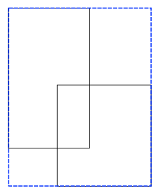
Let ${\mathcal{I}}_i=\{1,\dots ,i\}$ and $V\subseteq \tilde{V}$. Then $S(V,\tilde{V})$ is the ordered sequence whose $i$-th entry is the union of $V$ and the projections of $\tilde{V}$ onto the set of directions ${\mathcal{I}}_i$, i.e., $S(V,\tilde{V})$ is the ordered sequence of boxes from $V$ to $\tilde{V}$ by expanding in each direction. Let $\widetilde{c_i}$ denote the change in the cost function resulting from the expansion of $\tilde{V}$ in the one additional $i$-th direction.

Proposition 2.4

Let $V^l\supseteq V$, $V^k\supseteq V$, and $\hat{V}=V^l\cup V^k$ be expansions of a box $V$ such that $V=V^k\cap V^l$ for some neighborhood $N$. Let $S(V,V^l)$, $S(V,V^k)$, and $S(V,\hat{V})$ be the sequences with $c_i^1$, $c_i^k$, and $\widehat{c_i}$ being the corresponding changes in the cost function at the $i$-th step. Then

$$\sum _{i\in \mathcal{I}}\widehat{c_i}\le \sum _{i\in \mathcal{I}}(c_i^k+c_i^l).$$

One may imagine expanding from $V$ to $V^k$ to $\hat{V}$. The proposition is stating the corresponding total cost of this procedure is bounded above by the sum of each total cost of expansions $V^k$ and $V^l$ since the expansions are disjoint ($V=V^k\cap V^l$).

Theorem 2.5

The following results hold:

1. If $V^l,V^k\in {\text{Sol}}_{\alpha }(V,N)$, then $V^l\cap V^k\in {\text{Sol}}_{\alpha }(V,N)$
2. If $V^l,V^k\in {\text{Sol}}_{\alpha }(V,N)$, then $V^l\cup V^k\in {\text{Sol}}_{\alpha }(V,N)$

In other words, the union and intersection of two optimal solutions for the input box $V$ and neighborhood $N$ are also optimal solutions. For example, if $[a,c]$ and $[a,d]$ are optimal solutions such that $c\le d$ in Example 2.2 (the two points $a<b$ example), then both $[a,c]\cap [a,d]=[a,c]$ and $[a,c]\cup [a,d]=[a,d]$ are also optimal.

Theorem 2.6

Let $N=B(V,\pi )$ and $\tilde{N}=B(V,\tilde{\pi })$. If $\tilde{\pi }\ge \pi$ then

1. $C(V^l,\tilde{N})\le C(V^{\prime },\tilde{N})$ where $V^{\prime }\subseteq V^l$ and $V^l\in \text{Sol}(V,N)$
2. $C({\bigcap }_{V^l\in \text{Sol(V,N)}}{V}^l,\tilde{N})<C(V^{\prime },\tilde{N})$ where $V^{\prime }\subset {\bigcap }_{V^l\in \text{Sol}(V,N)}{V}^l$ and $V\subseteq V^{\prime }$
3. $\forall V^l\in \text{Sol}(V,N)$, $\exists V^k\in \text{Sol}(V,\tilde{N})$ such that $V^l\subseteq V^k$.
4. $\forall V^k\in \text{Sol}(V,\tilde{N})$, $\exists V^l\in \text{Sol}(V,N)$ such that $V^l\subseteq V^k$.

Interpretation of statements:

1. The cost of a subset of an optimal solution cannot be lower than the optimal solution even when the neighborhood is expanded.
2. The cost for a candidate solution that is strictly smaller than the intersection of all optimal solutions is strictly larger when the neighborhood is expanded.
3. When the neighborhood is enlarged, we get an optimal solution that contains the original optimal solution.

Lemma 2.7

The largest optimal solution of ${\text{Sol}}_{\alpha }(V,N)$ is contained in any $V^k\in {\text{Sol}}_{\tilde{\alpha }}(V,N)$ when $\tilde{\alpha }>\alpha$.

Lemma 2.8

Let $V^k\in {\text{Sol}}_{\alpha }(M,\Delta N)$ where $\Delta N=B(M,\tilde{\pi }-\pi )$ and $M\in {\text{Sol}}_{\alpha }(V,N)$ is a largest optimal solution. Then $V^k\in {\text{Sol}}_{\alpha }(V,\tilde{N})$.

Lemma 2.9

Let $M$ be a largest optimal solution in ${\text{Sol}}_{\alpha }(V,N)$ such that $M\ne V$. With $\gamma =(1/\alpha )-1$ we get that

$$\frac{\theta (N\backslash M)+\theta (\partial M)}{p}\ge \gamma \ge \frac{\theta (N\backslash M)}{q}$$

where $p,q\in \{1,\dots ,2n\}$ are the numbers of facets of $M$ that do not intersect $V$ and $N$, respectively.

If there are $m$ points in the neighborhood, the running time of the LP is $O(q^3\log q)$ where $q=mn$.

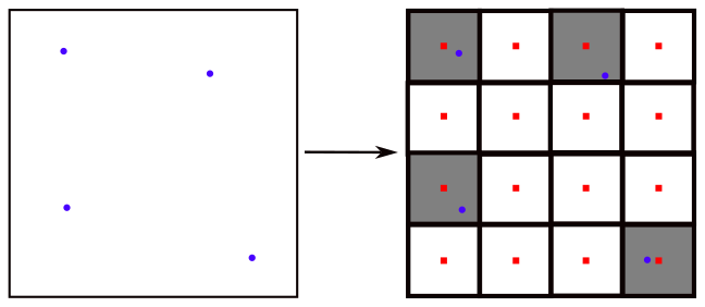
Pixel Cover

With the pixel cover we instead work over a discretization of $X\in {\mathbb{R}}^d$ where each pixel is a unit cube with integer vertices. We also assume that $\pi \in \mathbb{Z}$ when defining neighborhoods. All results shown above for point covers also hold true for pixel covers.

Define the integer ceiling by

$$\upharpoonright x\upharpoonleft =\{\begin{array}{ll}\lceil x\rceil & x\notin \mathbb{Z}\\ x+1& x\in \mathbb{Z}.\end{array}$$

For $x=(x_1,\dots ,x_n)\in X$ we define the pixel $\sigma =[\lfloor x_1\rfloor ],\upharpoonright x_1\upharpoonleft ]\times \cdots \times [\lfloor x_n\rfloor ,\upharpoonright x_n\upharpoonleft ]$ . We denote the centroid of a pixel $\sigma$ by $m_{\sigma }=(m_{\sigma }^1,\dots ,m_{\sigma }^n)$ and define $\theta (\sigma )$ to be the number of points in $X$ that are in $\sigma$. We denote by $\Theta (\tilde{V})$ the set of pixels $\sigma$ such that $m_{\sigma }\in \tilde{V}$ and $\theta (\sigma )\ne 0$, i.e., the set of nonempty pixels whose centroids are in the box $\tilde{V}$.

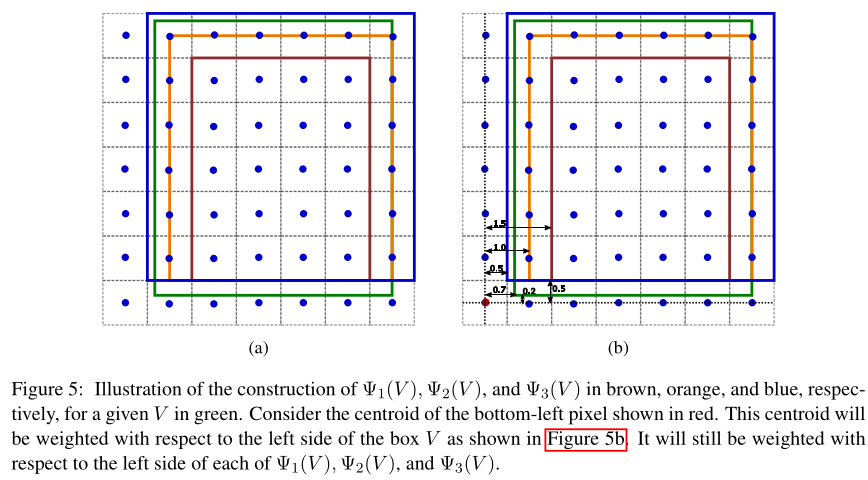
For a given input box $V$, let $\tilde{V}\supseteq V$ be a box in the neighborhood $N=B(V,\pi )$. The total width of box $\tilde{V}$ is given by $|\tilde{V}|={\sum }_{i\in \mathcal{I}}\widetilde{u_i}-\widetilde{l_i}$. Let $w_{\sigma }$ be the weight corresponding to pixel $\sigma \in \Theta (N)$ for a given expansion $\tilde{V}$,

$$w_{\sigma }\le \min \{\{m_{\sigma }^i-{\tilde{l}}^i\mid i\in \mathcal{I}\}\cup \{\widetilde{u_i}-m_{\sigma }^i\mid i\in \mathcal{I}\}\cup \{0.5\}\}.$$

Note that, like before, $m_{\sigma }\in \tilde{V}$ if and only if

$$\min \{\{m_{\sigma }^i-\widetilde{l_i}\mid i\in \mathcal{I}\}\cup \{\widetilde{u_i}-m_{\sigma }^i\mid i\in \mathcal{I}\}\}\ge 0.$$

For $V=[l_1,u_1]\times \cdots \times [l_n,u_n]$ we define the following LP:

$$\begin{array}{rlr}& \underset{\forall \tilde{V}\supseteq V}{\min }& {\overline{C}}_{\alpha }(\tilde{V},N)=-\alpha \sum _{\sigma \in \Theta (N)}{w}_{\sigma }\theta (\sigma )+(1-\alpha )\sum _{i\in \mathcal{I}}(\widetilde{u_i}-\widetilde{l_i})\\ & \text{subject to}& \widetilde{u_i}\ge u_i\forall i\in \{1,\dots ,n\}\\ & & \widetilde{l_i}\le l_i\forall i\in \{1,\dots ,n\}\\ & & w_{\sigma }\le m_{\sigma }^i-\widetilde{l_i}\forall i\in \{1,\dots ,n\},\sigma \in \Theta (N)\\ & & w_{\sigma }\le \widetilde{u_i}-m_{\sigma }^i\forall i\in \{1,\dots ,n\},\sigma \in \Theta (N)\\ & & w_{\sigma }\le 0.5\forall i\in \{1,\dots ,n\},\sigma \in \Theta (N)\end{array}$$

An optimal solution $[l_1^{\ast },u_1^{\ast }]\times \cdots \times [l_n^{\ast },u_n^{\ast }]\in {\overline{\text{Sol}}}_{\alpha }(V,N)$ may have non-integer coordinates. The paper claims that in such a case, there is another optimal solution with integer coordinates.

Recall that $\text{frac}(x)=x-\lfloor x\rfloor \in [0,1)$ is the fractional part of $x\in \mathbb{R}$.

Rounding Functions

Given a box $V=[l_1,u_1]\times \cdots \times [l_n,u_n]$ we define three rounded boxes ${\Psi }_r(V)=[{\psi }_r(l_1),{\psi }_r(u_1)]\times \cdots \times [{\psi }_r(l_n),{\psi }_r(u_n)]$ for $r=1,2,3$ where

$${\psi }_1(l_i)=\lceil l_i\rceil ,{\psi }_1(u_i)=\lfloor u_i\rfloor$$ $${\psi }_2(l_i)=\{\begin{array}{ll}\lceil l_i\rceil & \text{if }\text{frac}(l_i)\in (0.5,1)\\ \lfloor l_i\rfloor +0.5& \text{if }\text{frac}(l_i)\in (0,0.5]\\ \lfloor l_i\rfloor & \text{if }\text{frac}(l_i)=0\end{array},{\psi }_2(u_i)=\{\begin{array}{ll}\lfloor u_i\rfloor +0.5& \text{if }\text{frac}(u_i)\in [0.5,1)\\ \lfloor u_i\rfloor & \text{if }\text{frac}(u_i)\in [0,0.5)\end{array}$$ $${\psi }_3(l_i)=\{\begin{array}{ll}\lceil l_i\rceil & \text{if }\text{frac}(l_i)\in (0.5,1)\\ \lfloor l_i\rfloor & \text{if }\text{frac}(l_i)\in [0,0.5]\end{array},{\psi }_3(u_i)=\{\begin{array}{ll}\lceil u_i\rceil & \text{if }\text{frac}(u_i)\in [0.5,1)\\ \lfloor u_i\rfloor & \text{if }\text{frac}(u_i)\in [0,0.5)\end{array}$$