Multiple Correspondence Analysis

Multiple correspondence analysis (MCA) is a statistical technique for nominal data (categorical data without overlaps) that represents the data as points in low-dimensions. It is a counterpart to principle component analysis and an extension to correspondence analysis.

Correspondence Analysis

Correspondence analysis (CA) provides a means of displaying or summarizing a set of categorical data in two-dimensional graphical form. It is typically applied to a contingency table $C$ of a pair of nominal variables where each cell is a count or a zero value. An example of a contingency table is given below:

	Right-handed	Left-Handed	Total
Male	43	9	52
Female	44	4	48
Total	87	13	100

The first step before any computation is to transform the values in the matrix $C$. We start by computing a set of weights (called masses) for rows and columns:

$$w_m=\frac{1}{n_C}C\text{1}\text{ and }{w}_n=\frac{1}{n_C}{\text{1}}^{\top }C$$

where $\text{1}$ is the all-ones column vector and

$$n_C=\sum _{i=1}^n\sum _{j=1}^m{C}_{ij}.$$

We then construct diagonal matrices:

$$W_m=\text{diag}(1/\sqrt{w_m})\text{ and }{W}_n=\text{diag}(1/\sqrt{w_n}).$$

We then compute the matrix $S$, called the matrix of standardized residuals, by

$$S=W_m\left(P-w_m{w}_n\right)W_n$$

$P=C/n_C$ where $w_m{w}_n$ is the outer product.

We then perform singular value decomposition on $S$ to get

$$S=U\Sigma V^{\ast }$$

where $U$ and $V$ are the left and right unitary singular vectors of $S$ and $\Sigma$ is the diagonal matrix of singular values ${\sigma }_i$. $U$ is of dimension $m\times p$, $V$ is $n\times p$ and $\Sigma$ is of dimension $p\times p$ where $p\le \min (m,n)-1$.

We define the total inertia of the data table by

$$\text{I}=\sum _{i=1}^p{\sigma }_i^2$$

We want to transform the singular vectors to coordinates, forming the principal coordinates, while preserving the ${\chi }^2$-distances between rows or columns. For rows we use

$$F_m=W_{m}U\Sigma$$

and for columns we use

$$F_n=W_{n}V\Sigma .$$

Example

Consider the following contingency table, $C$:

	Tasty	Aesthetic	Economic
Butterbeer	5	7	2
Squishee	18	46	20
Slurm	19	29	39
Fizzy	12	40	49
Brawndo	3	7	16

Adding up the cells gives us that $n_C=312$. Resulting in a observed proportions table, $P$, of

	Tasty	Aesthetic	Economic
Butterbeer	0.016	0.022	0.006
Squishee	0.058	0.147	0.064
Slurm	0.061	0.093	0.125
Fizzy	0.038	0.128	0.157
Brawndo	0.01	0.022	0.051
We get a row masses of

$$w_m={\left[\begin{array}{ccccc}0.044& 0.269& 0.279& 0.324& 0.083\end{array}\right]}^{\top }$$

and column masses of

$$w_n=\left[\begin{array}{ccc}0.182& 0.413& 0.404\end{array}\right].$$

Computing the SVD of $S=W_m(P-w_m{w}_n)W_n$ results in the following data:

• Singular values ($\Sigma$):

1st dim	2nd dim	3rd dim
2.65e-01	1.14e-01	4.21e-17

• Left singular values ($U$):

	1st dim	2nd dim	3rd dim
Butterbeer	-0.439	-0.424	-0.326
Squishee	-0.651	0.355	0.029
Slurm	0.16	-0.672	-0.362
Fizzy	0.371	0.488	-0.747
Brawndo	0.466	-0.059	0.451

• Right singular values ($V$):

	1st dim	2nd dim	3rd dim
Tasty	-0.41	-0.806	0.427
Aesthetic	-0.489	0.59	0.643
Economic	0.77	-0.055	0.635
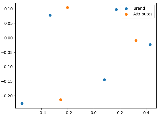
We can then compute the row principle coordinates ($F_m$):

	1st dim	2nd dim	3rd dim
Butterbeer	-5.49e-01	-2.271e-01	-1.009e-16
Squishee	-3.331e-01	7.768e-02	3.673e-18
Slurm	8.05e-02	-1.446e-01	-4.494e-17
Fizzy	1.73e-01	9.748e-02	-8.609e-17
Brawndo	4.305e-01	-2.352e-02	1.024e-16
and the column principle coordinates ($F_n$):

	1st dim	2nd dim	3rd dim
Tasty	-2.543e-01	-2.14e-01	6.555e-17
Aesthetic	-2.016e-01	1.041e-01	6.555e-17
Economic	3.215e-01	-9.751e-03	6.555e-17

Finally to visualize the results, we plot both coordinates with the first dimension on the $x$-axis and the second dimension on the $y$-axis:

Multiple Correspondence Analysis

MCA is performed by applying the CA algorithm to an indicator matrix (aka complete disjunctive table, see One-Hot Encoding). MCA only works on categorical data; any quantitative data (e.g. age, weight, height, etc) must be turned into categories through a method such as statistical quantiles.

Once the data set is only categorical, we construct the indicator matrix/table $X$. As a result, if there are $I$ observations and $K$ categorical variables where $J_k$ is the number of categories for the $k$-th variable, then $X$ is an $I\times J$ matrix with all coefficients being 0 or 1 where $J={\sum }_{k=1}^K{J}_k$.

We define $Z=X/N$ where $N$ is the sum of all entries of $X$. We construct two vectors:

$$r_i=\sum _{k=1}^I{Z}_{ki}\text{ and }{c}_i=\sum _{k=1}^J{Z}_{ik}$$

i.e., $r$ is the sums along the rows of $Z$ and $c$ is the sums along the columns of $Z$. We then find the singular value decomposition of

$$M=D_r^{-1/2}(Z-r{c}^{\top })D_c^{-1/2}$$

where $D_r=\text{diag}(r)$ and $D_c=\text{diag}(c)$. The SVD of $M$ gives us unitary matrices $U,V$ and diagonal matrix $\Sigma$ such that $M=U\Sigma V^{\ast }$. Then like before, we construct the row principle coordinates by

$$F=D_r^{-1/2}U\Sigma$$

and the column principle coordinates by

$$G=D_c^{-1/2}V\Sigma .$$

Interpreting Correspondence Plots

Correspondence analysis is about the relativistic relations. A correspondence analysis won’t show which rows/column have the maximum, instead it will tell you what categories had the most.

The distance from the origin is a measure of how discriminating a column is. Variables close to the origin typically have less distinct values.

Columns that are close together (ensure the plots aspect ratio is set to 1) is an indication of similarity between them. To compare the relationship between rows and columns you have to instead look for small angles between the line connecting them and the line to the origin.