Persistence stability for geometric complexes

Questions:

• Does the bottleneck metric require both persistence diagrams have the same number of points?
  • Answer: Unmatched points are projected down to the diagonal line. If we take into account the diagonal line, there is always the same number of points.
• The persistence modules work over a field $k$. The given example is homology groups over a field. Can this be done with homology groups over a group like ${\mathbb{Z}}_2$ or $\mathbb{Z}$?
  • Answer: Typically we work over a finite field ${\mathbb{Z}}_p$.
• How do persistence diagrams differ for persistence modules?
• Is it possible to construct an $ϵ$-interleaving?
  • Answer: It would be very difficult. Typically work with existence results.
• What exactly is $q$-tame modules?
• Proposition 3.3

Full paper can be found at: https://link.springer.com/article/10.1007/s10711-013-9937-z

A brief summary can be found at: 2024-09-06

Introduction

Given a metric space $(Y,d_Y)$ which “approximates” another metric space $(X,d_X)$, our goal is construct a simplicial complex on the vertex set $Y$ such that the homology or homotopy type is the same as $X$. In most applications, $Y$ is finite.

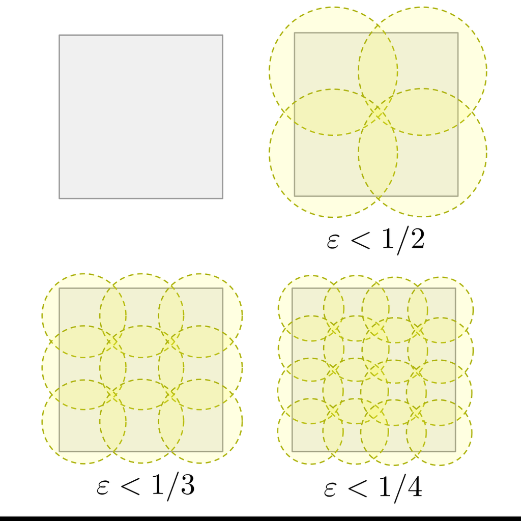
One common approach is simply the Vietoris-Rips complex:

$$\sigma =[x_0,x_1,\dots ,x_k]\in \text{Rips}(X,\alpha )\iff d_X(x_i,x_j)\le \alpha ,\forall i,j=0,1,\dots ,k.$$

For a closed Riemannian manifold $X$, the geometric realization of $\text{Rips}(X,\alpha )$ is homotopy equivalent for sufficiently small $\alpha$. More generally, if $(Y,d_Y)$ is “sufficiently close” (see daily note 2024-04-16 on Gromov-Hausdorff distance) to $(X,d_X)$, there is some $\alpha >0$ such that $\text{Rips}(Y,\alpha )$ is homotopy equivalent to $X$.

In summary, we can recover the underlying topology of $(X,d_X)$ from a sufficiently close approximation $(Y,d_Y)$. Unfortunately, finding the correct $\alpha$ as described above depends on the underlying geometry. We can circumnavigate this issue by using persistence of the filtration $\mathbb{R}\text{ips}(X)=(\text{Rips}(X,\alpha ){)}_{\alpha \in \mathbb{R}}$. It was shown by Chazal et al. that for finite metric spaces

$$d_b(\text{dgm}(\mathbb{R}\text{ips}(X)),\text{dgm}(\mathbb{R}\text{ips}(Y)))\le 2d_{GH}(X,Y)$$

where $d_b$ is the bottleneck metric on persistence diagrams and $d_{GH}$ is the Gromov-Hausdorff distance.

One immediate consequence of this result is that instead of working with the more messy Gromov-Hausdorff distance, we can use the bottleneck metric which is easier to compute.

Persistence modules and persistence diagrams

We define a persistence module $\mathbb{V}$ over $\mathbb{R}$ as an indexed family of vector spaces $(V_a{)}_{a\in \mathbb{R}}$ with a family of linear maps $(v_a^b:V_a\to V_b\mid a\le b)$ which satisfy $v_b^c\circ v_a^b=v_a^c$ whenever $a\le b\le c$.

$$\cdots \to V_a\stackrel{v_a^b}{\to }{V}_b\stackrel{v_b^c}{\to }{V}_c\to \cdots$$

Example: Let $\mathbb{S}=({\mathbb{S}}_a{)}_{a\in \mathbb{R}}$ be a filtered simplicial complex, that is, ${\mathbb{S}}_a\subset {\mathbb{S}}_b$ whenever $a\le b$. Let $V_a=H({\mathbb{S}}_a)$ be the homology groups (coefficients from a field $k$) and $v_a^b:V_a\to V_b$ be induced by inclusion ${\mathbb{S}}_a\hookrightarrow {\mathbb{S}}_b$. Then $(H({\mathbb{S}}_a){)}_{a\in \mathbb{R}}$ is a persistence module.

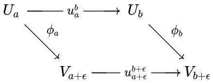
Given two persistence modules $\mathbb{U}$ and $\mathbb{V}$ over $\mathbb{R}$ and $ϵ\in \mathbb{R}$, we define a homomorphism of degree $ϵ$ as a collection $\Phi$ of linear maps

$$({\varphi }_a:U_a\to V_{a+ϵ}{)}_{a\in \mathbb{R}}$$

such that $v_{a+ϵ}^{b+ϵ}\circ {\varphi }_a={\varphi }_b\circ u_a^b$ whenever $a\le b$. In other words, the following diagram commutes.

We denote the set of such homomorphisms by ${\text{Hom}}^{ϵ}(\mathbb{U},\mathbb{V})$.

Example continued: Given $ϵ>0$, if $f:\overline{\mathbb{S}}\to {\overline{\mathbb{S}}}^{\prime }$ is a map between simplicial complexes such that ${\mathbb{S}}_a\mapsto {\mathbb{S}}_{a+ϵ}^{\prime }$ for any $a\in \mathbb{R}$, then $f$ induces a homomorphism between persistence modules $H(\mathbb{S})$ and $H({\mathbb{S}}^{\prime })$.

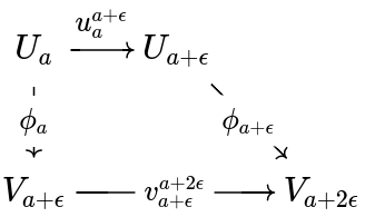
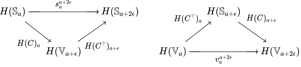
For $ϵ\ge 0$, an important $ϵ$-degree endomorphism is the shift map $1_{\mathbb{V}}^{ϵ}\in {\text{Hom}}^{ϵ}(\mathbb{V},\mathbb{V})$ given by the maps $(v_a^{a+ϵ}{)}_a$. One may see that for any $\Phi \in {\text{Hom}}^{ϵ}(\mathbb{U},\mathbb{V})$ we get that $\Phi 1_{\mathbb{U}}^{ϵ}=1_{\mathbb{V}}^{ϵ}\Phi$ for all $ϵ\ge 0$. That is, for all indices $a$ and $ϵ\ge 0$ the diagram below commutes:

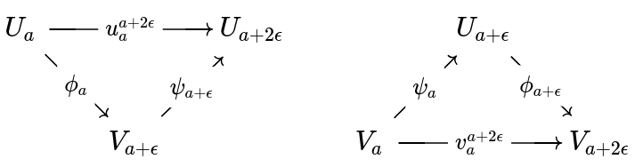
Two persistence modules are $ϵ$-interleaved if there are homomorphisms $\Phi \in {\text{Hom}}^{ϵ}(\mathbb{U},\mathbb{V})$ and $\Psi \in {\text{Hom}}^{ϵ}(\mathbb{V},\mathbb{U})$ such that $\Psi \Phi =1_{\mathbb{U}}^{2ϵ}$ and $\Phi \Psi =1_{\mathbb{V}}^{2ϵ}$. So for all indices $a$, the diagrams below commute:

Furthermore, a persistence module $\mathbb{V}$ is $q$-tame if $\text{rank}(v_a^b)<\infty$ whenever $a<b$.

Theorem 2.3

If $\mathbb{U}$ is a $q$-tame module then it has a well-defined persistence diagram $\text{dgm}(\mathbb{U})$. If $\mathbb{U},\mathbb{V}$ are $q$-tame persistence modules that are $ϵ$-interleaved then there exists an $ϵ$-matching between the multisets $\text{dgm}(\mathbb{U})$, $\text{dgm}(\mathbb{V})$. Thus, the bottleneck distance between them satisfies the bound $d_b(\text{dgm}(\mathbb{U}),\text{dgm}(\mathbb{V}))\le ϵ$.

In short, if two $q$-tame persistence modules are $ϵ$-interleaved then their bottleneck distance is less than $ϵ$. Since $d_b$ gives a lower-bound to the twice the Gromov-Hausdorff distance, $ϵ$-interleaved can be used to show two spaces are sufficiently close.

Multivalued maps

\epsilon-simplicial

Let $\mathbb{S}$ and $\mathbb{T}$ be two filtered simplicial complexes with vertex sets $X$ and $Y$ respectively. A map $f:X\to Y$ is $ϵ$-simplicial if it induces a simplicial map ${\mathbb{S}}_a\to {\mathbb{T}}_{a+ϵ}$ for every $a\in \mathbb{R}$. That is, for all simplices $\sigma \in {\mathbb{S}}_a$, we get $f(\sigma )\in {\mathbb{T}}_{a+ϵ}$ as a simplex.

The paper provides an unnecessarily complex definition of a multivalued map $C$ between $X$ and $Y$ as a subset of $X\times Y$ such that the projection $X\times Y\to X$ is surjective. Ultimately, the only difference is that a single $x\in X$ may be mapped to multiple $y\in Y$.

A single-valued map is subordinate to a multivalued map $C$ if $f(x)\in C(x)$ for all $x\in X$ and is denoted $f:X\stackrel{C}{\to }Y$.

\epsilon-simplicial

Let $\mathbb{S}$ and $\mathbb{T}$ be two filtered simplicial complexes with vertex sets $X$ and $Y$. A multivalued map $C:X\rightrightarrows Y$ is $ϵ$-simplicial if for any $a\in \mathbb{R}$ and any simplex $\sigma \in {\mathbb{S}}_a$, every finite subset of $C(\sigma )$ is a simplex of ${\mathbb{T}}_{a+ϵ}$.

Proposition 3.3

If $C$ is an $ϵ$-simplicial multivalued map, then $C$ induces a canonical linear map $H(C)\in {\text{Hom}}^{ϵ}(H(\mathbb{S}),H(\mathbb{T}))$ equal to $H(f)$ for any $f:X\stackrel{C}{\to }Y$.

Here $H(f)$ represents the homomorphism of degree $ϵ$ between $H(\mathbb{S})$ and $H(\mathbb{T})$ induced by $f$ (I think…). The proposition states that given any multivalued map $C$ that maps simplices in ${\mathbb{S}}_a$ to simplices in ${\mathbb{T}}_{a+ϵ}$, there is a homomorphism of degree $ϵ$ between $H(\mathbb{S})$ and $H(\mathbb{T})$. Moreover, it states that it is given by any subordinate map $f:X\stackrel{C}{\to }Y$ which implies that all subordinate maps induce the same homomorphism of degree $ϵ$. Thus, any subset of $C$, $C^{\prime }$ also gives the same map, i.e., $H(C)=H(C^{\prime })$ for any multivalued map $C^{\prime }\subset C$.

Proposition 3.5

Let $\mathbb{S},\mathbb{T},\mathbb{U}$ be filtered complexes with vertex sets $X,Y,Z$. If

• $C:X\rightrightarrows Y$ is $ϵ$-simplicial
• $D:Y\rightrightarrows Z$ is $\delta$-simplicial

then $D\circ C:X\rightrightarrows Z$ is $(ϵ+\delta )$-simplicial and $H(D\circ C)=H(D)\circ H(C)$.

Correspondences

Correspondence

A multivalued map $C:X\rightrightarrows Y$ is a correspondence if the projection $C\to Y$ is surjective, i.e., for every $y\in Y$ there is at least one $x\in X$ such that $(x,y)\in C$. Alternatively, the transpose $C^{\top }$ (constructed by image of $(x,y)\mapsto (y,x)$ map) is a multivalued map.

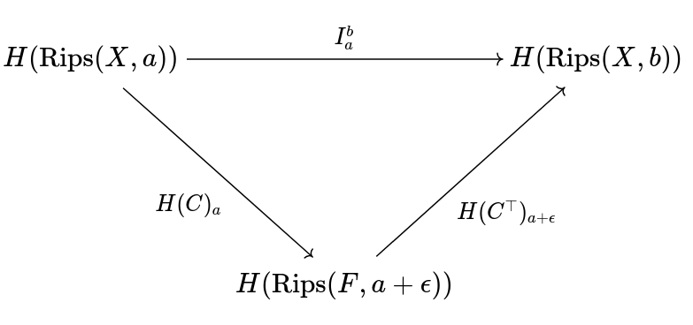
If $C$ is a correspondence then the maps $1_X=\{(x,x)\}$ and $1_Y=\{(y,y)\}$ satisfy

$$1_X\subset C^{\top }\circ C\text{ and }{1}_Y\subset C\circ C^{\top }.$$

Let $C$ be a correspondence between vertex sets of filtered complexes $\mathbb{S}$ and $\mathbb{V}$. If $C$ maps simplices $\sigma \in {\mathbb{S}}_a$ to simplices $C(\sigma )\in {\mathbb{V}}_{a+ϵ}$ and $C^{\top }$ maps simplices $\tau \in {\mathbb{V}}_a$ to simplices $C^{\top }(\tau )\in {\mathbb{S}}_{a+ϵ}$, then $H(C)$ and $H(C^{\top })$ induce $ϵ$-interleaved persistence modules $H(\mathbb{S})$ and $H(\mathbb{V})$.

Proposition 4.2

Let $\mathbb{S}$, $\mathbb{T}$ be filtered complexes with vertex sets $X$, $Y$. If $C:X\rightrightarrows Y$ is a correspondence such that $C$ and $C^{\top }$ are both $ϵ$-simplicial, then they induce a $ϵ$-interleaving between $H(\mathbb{S})$ and $H(\mathbb{T})$, namely $H(C)$ and $H(C^{\top })$.

Proposition 4.2 and Theorem 2.3 lay out a foundation for proving an upper bound on the bottleneck distance. That is, showing the filtered complexes are $q$-tame and there is a correspondence $C$ such that $C$ and $C^{\top }$ are $ϵ$-simplicial.

Consider the case where $X$ and $Y$ are metric spaces. Then a correspondence $C:X\rightrightarrows Y$ has distortion defined by

$$\text{dis}(C)=\sup \{|d_X(x,x^{\prime })-d_Y(y,y^{\prime })|:(x,y),(x^{\prime },y^{\prime })\in C\}.$$

We can us the distortion to calculate the Gromov-Hausdorff distance:

$$d_{GH}(X,Y)=\frac{1}{2}\inf \{\text{dis}(C):C:X\rightrightarrows Y\text{ is a correspondence}\}.$$

“low-distrortion” correspondences give rise to $ϵ$-simplicial maps.

Vietoris-Rips and Cech complex

Let $(X,d_X)$ be a metric space. We get a filtered simplicial complex $\mathbb{R}\text{ips}(X)=(\text{Rips}(X,a){)}_{a\in \mathbb{R}}$ where

$$[x_0,x_1,\dots ,x_k]\in \text{Rips}(X,a)\iff d_X(x_i,x_j)\le a\text{ for all }i,j.$$

Lemma 4.3

Let $(X,d_X)$ and $(Y,d_Y)$ be metric spaces. For any $ϵ>2d_{GH}(X,Y)$ the persistence modules $H(\mathbb{R}\text{ips}(X))$ and $H(\mathbb{R}\text{ips}(Y))$ are $ϵ$-interleaved.

Since $ϵ>2d_{GH}$ there is a correspondence $C:X\rightrightarrows Y$ with distortion at most $ϵ$. Consider $\sigma \in \text{Rips}(X,a)$ and finite subset $\tau \subset C(\sigma )$. Notice that for any $y,y^{\prime }\in \tau$, there is some $x,x^{\prime }\in \sigma$ such that $y\in C(x)$ and $y^{\prime }\in C(x^{\prime })$. Then

$$|d_X(x,x^{\prime })-d_Y(y,y^{\prime })|\le ϵ.$$

But by the reverse-triangle inequality,

$$d_Y(y,y^{\prime })\le d_X(x,x^{\prime })+ϵ\le a+ϵ$$

So $\tau \in \text{Rips}(Y,a+ϵ)$. Thus, $C$ is an $ϵ$-simplicial from $\mathbb{R}\text{ips}(X)$ to $\mathbb{R}\text{ips}(Y)$. A similar argument holds for $C^{\top }$.

The paper proves a similar result for the Cech complex.

Dowker Complexes

The Cech complex discussed in class is known as the “intrinsic Cech complex” and is constructed from a single metric space. A common approach in TDA is to use a pair or triple of metric spaces. These are examples of a more general class known as Dowker Complex.

Let $L$ and $W$ be subsets representing ‘landmarks’ and ‘witnesses’ of a metric space. For $a\in \mathbb{R}$ the ambient Cech complex has vertices $L$ and simplices given by

$$\sigma \in \text{Cˇech}(L,W,a)\iff \exists w\in W\text{ such that }d(w,l)\le a\text{ for all }l\in \sigma .$$

Letting $a\to \infty$ gives a filtered complex $\mathbb{C}\text{ech}(L,W)$.

This varies from the intrinsic Cech complex by only including $n$-simplices if the intersection of the $(n+1)$-balls include a witness point. One may see that the intrinsic Cech complex is simply the ambient Cech complex with ${\mathbb{R}}^n$ as the witness set.

Let $L$ and $W$ be sets and $\Lambda :L\times W\to \mathbb{R}$ a function. For $a\in \mathbb{R}$ the Dowker complex has vertices $L$ and simplices given by

$$\sigma \in \text{Dow}(\Lambda ,a)\iff \exists w\in W\text{ such that }\Lambda (l,w)\le a\text{ for all }l\in \sigma .$$

Likewise, letting $a\to \infty$ gives a filtered complex $\mathbb{D}\text{ow}(\Lambda )$. Notice that for a metric space $(X,d_X)$, $\mathbb{C}\text{ech}(X)$ is the same as $\mathbb{D}\text{ow}(d_X)$. Likewise, the ambient Cech complex $\mathbb{C}\text{ech}(L,W)$ is the same as $\mathbb{D}\text{ow}(d{\mid }_{L\times W})$ where $(X,d)$ is the ambient space.

We compare two sets of data $(L,W,\Lambda )$ and $(L^{\prime },W^{\prime },{\Lambda }^{\prime })$ with correspondences $C:L\rightrightarrows L^{\prime }$ and $D:W\rightrightarrows W^{\prime }$ and define their distortion by

$$\text{dis}(C,D)=\underset{(l,l^{\prime })\in C}{\sup }\underset{(w,w^{\prime })\in D}{\sup }|\Lambda (l,w)-{\Lambda }^{\prime }(l^{\prime },w^{\prime })|.$$

Lemma 4.9

If $C:L\rightrightarrows L^{\prime }$ and $D:W\rightrightarrows W^{\prime }$ are correspondences and $ϵ\ge \text{dis}(C,D)$ then the persistence modules $H(\mathbb{D}\text{ow}(\Lambda ))$ and $H(\mathbb{D}\text{ow}({\Lambda }^{\prime }))$ are $ϵ$-interleaved.

The proof is almost identical to the Vietrois-Rips interleaving.

Corollary 4.10

Let $d_H$ denote the Hausdorff distance between subsets of a metric space. For any $ϵ>d_H(L,L^{\prime })$ the ambient Cech persistence modules $H(\mathbb{C}\text{ech}(L,W))$ and $H(\mathbb{C}\text{ech}(L^{\prime },W^{\prime }))$ are $ϵ$-interleaved.

Witness Complex

The paper generalized the Witness Complex discussed in class from the Euclidean metric to an arbitrary function $\Lambda :L\times W\to \mathbb{R}$. Then for any $\sigma \subset L$, $w\in W$ and $a\in \mathbb{R}$, we say $w$ is an $a$-witness for simplex $\sigma$ if

$$\Lambda (l,w)\le \Lambda (l^{\prime },w)+a\text{ for all }l\in \sigma \text{ and }{l}^{\prime }\in L\backslash \sigma .$$

Thus,

$$\sigma \in \text{Wit}(L,W;a)\iff \forall \tau \subseteq \sigma ,\exists w\in W\text{ such that w is an a-witness for }\tau .$$

Clearly $\text{Wit}(L,W;a)\subset \text{Wit}(L,W;b)$ for $a<b$. Thus, by inclusion maps we get a filtered simplicial complex $\mathbb{W}\text{it}(L,W)$.

Let $W$ and $W^{\prime }$ be two witness sets for $L$ with maps $\Lambda :L\times W\to \mathbb{R}$ and ${\Lambda }^{\prime }:L\times W^{\prime }\to \mathbb{R}$. Then the distortion of a correspondence $C:W\rightrightarrows W^{\prime }$ is given by

$$\text{dis}(C)=\underset{l\in L}{\sup }\underset{(w,w^{\prime })\in C}{\sup }|\Lambda (l,w)-{\Lambda }^{\prime }(l,w^{\prime })|.$$

If $ϵ\ge 2\text{dis}(C)$, then $H(\mathbb{W}\text{it}(L,W))$ and $H(\mathbb{W}\text{it}(L,W^{\prime }))$ are $ϵ$-interleaved. The proof follows a similar pattern as for Vietoris-Rips.

Often with witness complexes, $L$ and $W$ come from an ambient metric space and $\Lambda =d{|}_{L\times W}$ (see class notes). In such a situation, if $ϵ>2d_H(W,W^{\prime })$ then the persistence modules $H(\mathbb{W}\text{it}(L,W))$ and $H(\mathbb{W}\text{it}(L,W^{\prime }))$ are $ϵ$-interleaved. This is a corollary of the previous result. The set

$$C=\{(w,w^{\prime })\in W\times W^{\prime }:d_X(w,w^{\prime })<\frac{1}{2}ϵ\}$$

forms a correspondence with $\text{dis}(C)\le \frac{1}{2}ϵ$.

Remark: The above results do not apply when the two spaces have differing landmark sets.

Counterexample: Let $W=L=\{0,1\}\subset \mathbb{R}$ and $L^{\prime }=\{-\delta ,0,1,1+\delta \}$ for some $\delta \in (0,1/2)$. Then

$$\text{Wit}(L,W;a)=\{[0],[1],[0,1]\}\text{ for all }a\ge 0$$

whereas

$$\text{Wit}(L^{\prime },W;a)=\{[-\delta ],[0],[1],[1+\delta ],[-\delta ,0],[1,1+\delta ]\}$$

for all $a\in [\delta ,1-\delta )$. Even though $d_H(L,L^{\prime })=\delta$ can be made arbitrarily small, the homology persistence modules do not $ϵ$-interleave when $ϵ<1-2\delta$.

Regularity of Rips and Cech filtrations

A subset $F\subset X$ of a metric space $(X,d_X)$ is an $ϵ$-sample of $X$ if for any $x\in X$, there is some $f\in F$ such that $d_X(x,f)<ϵ$. In other words, every point in $X$ can be approximated by a point in $F$. We say a metric space $(X,d_X)$ is totally bounded if it has a finite $ϵ$-sample for every $ϵ>0$. Alternatively $X$ is totally bounded if for every $ϵ>0$ we can cover $X$ with finitely many balls. For example, a bounded subset in ${\mathbb{R}}^n$ would be totally bounded.

Proposition 5.1

If $(X,d_X)$ is a totally bounded metric space then the persistence modules $H(\mathbb{R}\text{ips}(X))$ and $H(\mathbb{C}\text{ech}(X))$ are $q$-tame.

The proof constructs the correpondence: $C=\{(x,f)\in X\times F:d_X(x,f)<\frac{1}{2}ϵ\}$ where $F$ is an $\frac{1}{2}ϵ$ sample of $X$. Notice that for all $(x,f),(x^{\prime },f^{\prime })\in C$,

$$\begin{array}{rl}|d_X(x,x^{\prime })-d_X(f,f^{\prime })|& \le |d_X(x,x^{\prime })-d_X(x,f^{\prime })|+|d_X(x,f^{\prime })-d_X(f,f^{\prime })|\\ & \le d_X(x^{\prime },f^{\prime })+d_X(x,f)\\ & <ϵ.\end{array}$$

As a result, the Gromov-Hausdorff distance is less than $\frac{1}{2}ϵ$ and there is an $ϵ$-interleaving (Lemma 4.3). Letting $ϵ=(b-a)/2$ results in the map $I_a^b$ in the persistence module factoring into Since $F$ is finite-dimensional, $\text{Rips}(F,a+ϵ)$ is a finite simplicial complex. Therefore, $I_a^b$ has finite rank.

As a result the persistence diagrams of $H(\mathbb{R}\text{ips}(X))$ and $H(\mathbb{C}\text{ech}(X))$ are well-defined for totally bounded metric spaces.

Theorem 5.2

Let $X,Y$ be totally bounded metric spaces. Then

$$d_b(\text{dgm}(H(\mathbb{R}\text{ips}(X))),\text{dgm}(H(\mathbb{R}\text{ips}(Y))))\le 2d_{GH}(X,Y)$$

and

$$d_b(\text{dgm}(H(\mathbb{C}\text{ech}(X))),\text{dgm}(H(\mathbb{C}\text{ech}(Y))))\le 2d_{GH}(X,Y).$$

Proof: Lemma 4.3, Proposition 5.1, and Theorem 2.3.

We get similar results for ambient Cech complexes:

Proposition 5.4

Let $L,W$ be subsets of a metric space. If at least one of $L,W$ is totally bounded, then the ambient Cech persistence $H(\mathbb{C}\text{ech}(L,W))$ is $q$-tame.

The proof is similar to proposition 5.1. For every $ϵ>0$ it shows that $H(\mathbb{C}\text{ech}(L,W))$ is $ϵ$-interleaved with a finite simplicial complex. Namely, $H(\mathbb{C}\text{ech}(F,W))$ where $F$ is an $ϵ$-sample with $d_H(L,F)\le ϵ$.

Theorem 5.6

Let $L,L^{\prime }$ and $W$ be subsets of a metric space. Suppose $L,L^{\prime }$ are totally bounded or that $W$ is totally bounded. Then

$$d_b(\text{dgm}(H(\mathbb{C}\text{ech}(L,W))),\text{dgm}(H(\mathbb{C}\text{ech}(L^{\prime },W))))\le d_H(L,L^{\prime }).$$

Finally for Dowker complexes:

Proposition 5.7

Let $L,W$ be sets and $\Lambda :L\times W\to \mathbb{R}$ be a function. Suppose the collection $({\lambda }_l{)}_{l\in L}$ of functions ${\lambda }_l(w)=\Lambda (l,w)$ is bounded and totally bounded with respect to the supremum norm on functions $W\to \mathbb{R}$. Then $H(\mathbb{D}\text{ow}(\Lambda ))$ is $q$-tame.

Again we show that $H(\mathbb{D}\text{(}ow)(\Lambda ))$ is $ϵ$-interleaved with a persistent homology for a finite simplicial complex. Let $F$ be a finite subset of $L$ such that $({\lambda }_l{)}_{l\in F}$ is an $ϵ$-sample of $({\lambda }_l{)}_{l\in L}$. Construct the following correspondences:

$$C=\{(l,l^{\prime })\in L\times F\mid \Vert {\lambda }_l-{\lambda }_{l^{\prime }}{\Vert }_{\infty }<ϵ\}$$ $$D=\{(w,w)\mid w\in W\}$$

By Lemma 4.9, we get that $H(\mathbb{D}\text{ow}(\Lambda ))$ and $H(\mathbb{D}\text{ow}({\Lambda }_F))$ are $ϵ$-interleaved.

The homology groups of a Rips filtration

One may construct a homology group $H_1(\text{Rips}(X,a))$ with uncountable infinite dimension.

Let

$$X=\{(t,0)\in {\mathbb{R}}^2:t\in [0,1]\}\cup \{(t,1)\in {\mathbb{R}}^2:t\in [0,1]\}$$

with the metric from ${\mathbb{R}}^2$. Notice that for any $t\in [0,1]$, the edge $e_t=[(t,0),(t,1)]$ is in $\text{Rips}(X,1)$ but no triangles contain $e_t$ in its boundary. Thus, for each $t\in (0,1]$, the cycles

$${\gamma }_t=[(0,0),(t,0)]+e_t+[(t,1),(0,1)]-e_0$$

form a linearly independent set in $H_1(\text{Rips}(X,1))$.

Here the filtration is only “bad” for a single radius ($r=1$). The paper provides a construction with arbitrarily large “bad” radii.

Proposition 5.9

For any $\alpha ,\beta \in \mathbb{R}$ with $0<\alpha \le \beta$ and integer $k$, there is a compact metric space $X$ such that for any $a\in [\alpha ,\beta ]$ the $k$-homology $H_k(\text{Rips}(X,a))$ has an uncountable infinite dimension.

The assumes $\alpha =1$ and $\beta =2$ (why?) and begins with the case $k=1$. It constructs the following space:

$$X=\{(t,0,z)\in {\mathbb{R}}^3:t\in [0,2],z\in [0,1]\}\cup \{(t,1+\frac{t}{2},z)\in {\mathbb{R}}^3:t\in [0,2],z\in [0,1]\}$$

with the ${\ell }^1$ norm in ${\mathbb{R}}^3$.

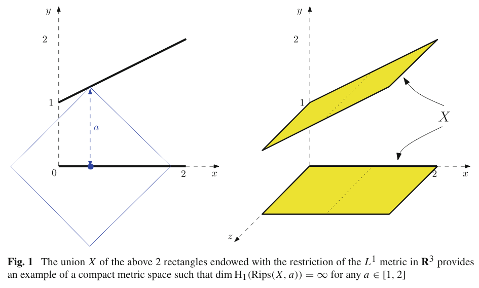
For $a\in [1,2]$ and $z\in [0,1]$ the edge $e_z=[(2(a-1),0,z),(2(a-1),a,z)]$ is in $\text{Rips}(X,a)$ but not contained in any non-degenerate triangle. Thus, for $z\in (0,1]$ the cycles

$${\gamma }_z=[(2(a-1),0,0),(2(a-1),0,z)]+e_z+[(2(a-1),a,z),(2(a-1),a,0)]-e_0$$

are not homologous to 0 and linearly independent.

For $k>1$, we take the product of $X$ with a $(k-1)$-dimensional sphere with sufficiently large radius. It then follows by Künneth theorem:

$$\underset{i+j=k}{⨁}{H}_i(X)\otimes H_j(Y)\cong H_k(X\times Y).$$

The open Vietoris-Rips filtration

The Vietoris-Rips complex uses closed balls which was crucial to our “bad” constructions. We consider the open Vietoris-Rips complex made with open balls:

$$[x_0,x_1,\dots ,x_k]\in \text{Rips}(X,a^{-})\iff d_X(x_i,x_j)<a\text{ for all }i,j.$$

Under the open Vietoris-Rips complex the bad edge no longer exists. Under this construction we can ensure at least the homology is countable.

Proposition 5.10

For any totally bounded metric space $X$ and real number $a>0$, the total homology $H(\text{Rips}(X,a^{-}))$ has a countable basis.

Any cycle in $H_k(\text{Rips}(X,a^{-}))$ is a finite linear combination of simplices with diameter less than $a$. Thus, there is some $n$ such that their diameter is less than $a-1/n$. Notice that such a class lives in the image of $H_k(\text{Rips}(X,a-1/n))\to H_k(\text{Rips}(X,a))$. By proposition 5.1, $H_k(\mathbb{R}\text{ips}(X))$ is $q$-tame. So this image is finite dimensional. Moreover, $H_k(\text{Rips}(X,a))$ is the union of all such images as $n\to \infty$. Since each image is finite, $H_k(\text{Rips}(X,a))$ must have a countable basis.

However, we cannot guarantee finiteness.

Proposition 5.11

For any given $a>0$ there exists a totally bounded metric space $X$ such that $H_1(\text{Rips}(X,a^{-}))$ has infinite dimension.

The first homology group of a Cech filtration

While the homology groups $H_k(\text{Cech}(X,a))$ can be infinite dimensional for $k\ge 2$, the first homology group is better behaved.

Proposition 5.12

Let $(X,d)$ be a totally bounded metric space, and let $a\ge 0$. Then over any coefficient ring $A$ and any $a\in \mathbb{R}$, $H_1(\text{Cech}(X,a),A)$ is finitely generated over $A$. In particular, if $A$ is a field $k$ then ${\dim }_k(H_1(\text{Cech}(X,a),k))<\infty .$

Proof sketch:

1. Every 1-cycle is homologous to a 1-cycle whose edges are at most length $a$
2. There is a finite set of edges $E_a$ with length at most $a$ such that for any edge $[x,y]$ of length at most $a$, there is an edge $[x^{\prime },y^{\prime }]$ in $E_a$ such that $d(x,x^{\prime })\le a$ and $d(y,y^{\prime })\le a$.
3. Any 1-cycle can be written in the form $[x_1,x_2]+[x_2,x_3]+\cdots +[x_k,x_1]$
4. Any 1-cycle $\gamma$ of the form $\gamma =[x_1,x_2]+[x_2,x_3]+\cdots +[x_k,x_1]$ with edges having length at most $a$ is homologous to cycle whose edges are in $E_a$.
5. Since every 1-cycle involves a finite set of edges $E_a$, the first homology group is finitely generated.

Special classes of metric spaces