Improving Mapper's Robustness by Varying Resolution According to Lens-Space Density

Authors: Kaleb Ruscitti and Leland McInnes

Full paper can be found at https://arxiv.org/abs/2410.03862.

---

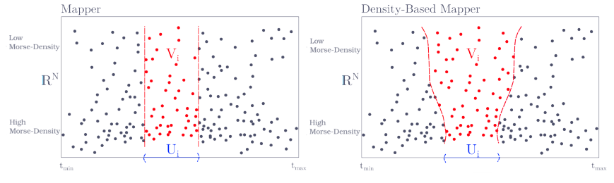
Recall that in the typical application of Mapper, we first project the data onto the real line. We then cover the real-line with uniform size intervals whose size we call the resolution $r>0$. Mapper is sensitive to the resolution, which determines the scale of topological features the Mapper can detect. Finding the choice for $r$ can be difficult apriori.

Typically the resolution is a global parameter that is fixed across the entire sample. The authors propose an improvement to Mapper by using a locally-varying choice of resolution. They provide a methodology of computing said variation from the data set.

Density Based Mapper

Herein, we denote by ${\mathbb{X}}_n$ samples taken from some distribution on a topological space $X$ with known pairwise distances and Morse-type function $f:X\to \mathbb{R}$.

Morse-type

A continuous real-valued function $f$ on a topological space $X$ is of Morse type if:

1. There is a finite set $\text{Crit}(f)=\{a_1<\cdots <a_n\}$, called the set of critical values, such that over every open interval $(a_0=-\infty ,a_1),\dots ,(a_i,a_{i+1}),\dots ,(a_n,a_{n+1}=+\infty )$ there is a compact and locally connected space $Y_i$ and a homeomorphism ${\mu }_i:Y_i\times (a_i,a_{i+1})\to X^{(a_i,a_{i+1})}$ such that $\forall i=0,\dots ,n$, $f|-X^{(a_i,a_{i+1})}={\pi }_2\circ {\mu }_i^{-1}$ where ${\pi }_2$ is the projection onto the second factor;
2. $\forall i=1,\dots ,n-1$, ${\mu }_i$ extends to a continuous function $\overline{{\mu }_i}:Y_i\times [a_i,a_{i+1}]\to X^{[a_i,a_{i+1}]}$;
3. Each levelset $X^t$ has a finitely generated homology.

Kernel Perspective on Mapper

Let $\mathcal{U}=\{U_i{\}}_{i=1}^N$ be a finite open cover of $f({\mathbb{X}}_n)$, then the pullback cover of ${\mathbb{X}}_n$ is $\mathcal{V}=\{f^{-1}(U_i){\}}_{i=1}^N$. We cluster each pullback $f^{-1}(U_i)$ and label the clusters $\{v_j^i{\}}_{j=1}^{J_i}$. Then the Mapper graph has vertices

$$V(G)=\bigcup _{i=1}^N\{v_j^i{\}}_{j=1}^{J_i}$$

and edges

$$E(G)=\bigcup _{i=1}^{N-1}\{(v_j^i,v_{j^{\prime }}^{i+1})\mid v_j^i\cap v_{j^{\prime }}^{i+1}\ne \varnothing \}.$$

Let ${\chi }_i:\mathbb{R}\to \{0,1\}$ be the characteristic function of $U_i$, i.e., ${\chi }_i(t)=1$ if and only if $t\in U_i$. Then $f^{-1}(U_i)=f^{-1}({\chi }_i^{-1}(1))$.

Thus, one may generalize the Mapper by defining new kernel functions $K$.

For example, if $U_i=(m_i-w/2,m_i+w/2)$, then the kernel function $K_i:{\mathbb{X}}_n\to \mathbb{R}$ given by

$$K_i(x)=\{\begin{array}{ll}1& \text{if }|f(x)-m_i|<w/2\\ 0& \text{otherwise}\end{array}$$

gives $f^{-1}(U_i)=K_i^{-1}(1)$.

Density-Sensitive Kerneled Covers

We wish to construct a Mapper which is sensitive to density information of ${\mathbb{X}}_n$.

f-kernel

An $f$-kernel function $K:X\times \mathbb{R}\to \mathbb{R}$ centered at $t_0\in L$ is a function such that:

1. If $f(x)=t_0$ then $K(x,t_0)=1$
2. $K$ is continuous on the set $\{x\in X\mid K(x,\rho )>0\}\subset X$.
3. For a fixed $t_0$, $K(x,t_0)$ is monotone non-increasing in $|f(x)-t_0|$. [UNCLEAR]

For a fixed $r>0$, we say that a choice of kernel $K$ and $ϵ>0$ has sufficient width if $|f(x)-t_0|<r⟹K(x,t_0)>ϵ$.

For example, the function $K:X\times \mathbb{R}\to \mathbb{R}$ given by

$$K(x,t_0)=\exp \left[\log (ϵ)(f(x)-t_0{)}^2\right]$$

is a $f$-kernel function centered at $t_0\in \mathbb{R}$. This kernel centered at 0 is drawn below:

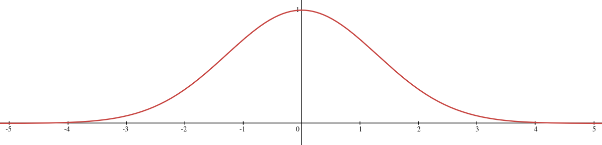
Notice that if $|f(x)-t_0|<1$, then

$$K(x,t_0)=\exp [\log (ϵ)(f(x)-t_0{)}^2]>\exp [\log (ϵ)]=ϵ,$$

i.e., for $r=1$ the kernel $K$ has sufficient width.

Let $\mathcal{U}$ be a generic open maximal interval cover (gomic for short) of $L=[t_{min},t_{max}]$, i.e., a cover of open intervals where no more than two intervals intersect at a time and the overlap $g$ defined by

$$g:=\frac{\ell (U_i\cap U_j)}{\ell (U_i)}$$

where $\ell$ is the Lebesgue measure satisfies $g\in (0,1)$ for all $U_i\cap U_j\ne \varnothing$.

For each interval $U_i\in \mathcal{U}$ let $m_i\in U_i$ be its midpoint. We say a family of kernel functions $\{K_i{\}}_{i=1}^N$ has sufficient width relative to $\mathcal{U}$ for threshold $ϵ>0$ if $K_i$ centered at $m_i\in U_i$ has sufficient width with radius $\ell (U_i)/2$ for every $U_i\in \mathcal{U}$.

Def

Given $(X,f)$, $\mathcal{U}$ and $K=\{K_i{\}}_{i=1}^N$ as above, the kerneled cover of $X$ associated to $(\mathcal{U},K)$, with threshold $ϵ>0$, is the cover $\mathcal{V}$ consisting of sets

$$V_i:=K_i^{-1}(ϵ,\infty )$$

for every $i=1,\dots ,N$.

Question: Are we defining the family of kernels as $K_i(x)=K(x,m_i)$?

Prp

Let $\mathcal{U}$ be an open cover of ${\mathbb{R}}^n$ consisting of open balls $B(r_i,t_i)$. Let $\mathcal{V}$ be the kerneled cover for $(\mathcal{U},K)$ with threshold $ϵ$. If the $\{K_i\}$ have sufficient width relative to $\mathcal{U}$, then $\mathcal{V}$ is an open cover of $X$.

Proof: Since $K$ is continuous, $V_i=K_i^{-1}(ϵ,\infty )$ is open. By the sufficient width condition, if $x\in f^{-1}(U_i)$ then $|f(x)-t_0|<r_i$ which implies that $K(x,f(x))>ϵ$ so $f^{-1}(U_i)\subset V_i$. Hence,

$$X\subset \bigcup _{i\in I}{f}^{-1}(U_i)\subset \bigcup _{i\in I}{V}_i.\text{\hspace{1em}□}$$

Let $\beta (x)$ be the distance in $L$ from $x$ to its $k$th nearest neighbor in $X$. We define $c(\beta ):[0,\infty )\to [1,c_{max}]$ to be a normalized sigmoid function,

$$c(\beta )=c_{max}\left(1+\exp \left[\frac{-(\beta -\mu )}{\sigma }\right]\right),$$

where $\mu ,\sigma$ are the mean and standard deviation of $\beta (x)$ respectively.

Prp

Suppose $K(x,t_0)=\exp \left[\frac{2\log (ϵ)}{r^2}c(\beta )\frac{(f(x)-t_0^2)}{2}\right]$ is the kernel function associated to the open ball $B(r,t_0)$. Then $K(x,t_0)$ has sufficient width for threshold $ϵ$.

Proof: Assume that $|f(x)-t_0|<r$. Then since $c(\beta )\ge 1$,

$$K(x,t_0)=\exp \left[\frac{2\log (ϵ}{r^2}c(\beta )\frac{(f(x)-t_0{)}^2}{2}\right]>\exp \left[\frac{2\log (ϵ)}{r^2}\frac{r^2}{2}\right]=ϵ\text{\hspace{1em}□}$$

This kernel was found by taking the Gaussian kernel $K(x,t_0)\propto \exp (c(\beta )(f(x)-t_0{)}^2)$ and solving for a normalizing constant which guarantees sufficient width.

Def

Let $\mathcal{V}$ be an open cover of a manifold $X$, with Morse-type function $f:X\to L\subset \mathbb{R}$. Let the resolution of $\mathcal{V}$ be

$$r=\underset{V\in \mathcal{V}}{\sup }\left(\underset{x,y\in V}{\sup }|f(x)-f(y)|\right).$$

When $\mathcal{V}$ is the pullback under $f$ of an open cover $\mathcal{U}$ for $L$, this reduces to the resolution of the regular Mapper, $r={\sup }_{U\in \mathcal{U}}\ell (U)$.

Density-Based Mapper Algorithm

Let ${\mathbb{X}}_n\subset {\mathbb{R}}^d$ be a set of samples, and let $\{t_1,\dots ,t_n\}$ denote the associated values of $f$. Fix a clustering algorithm and parameters $k$ (number of nearest neighbors to find), $N$ (number of cover elements), $g\in (0,1)$ (cover overlap) and an $f$-kernel function $K$. The algorithm has the following steps:

1. Compute the inverse approximate Morse density $\beta (x)$ for $x\in {\mathbb{X}}_n$.
2. Determine an open cover of intervals $\mathcal{U}=\{U_i=B(w_i,t_i){\}}_{i=1}^N$ that have overlap $g$.
3. For each interval $U_i$
   1. Compute the kernel $K(x,t_i)$ for each $x\in {\mathbb{X}}_n$ and define $V_i=\{x\mid K(x,t_i)>ϵ\}$.
   2. Run the clustering algorithm to assign each point in $V_i$ a cluster label $c_i(x)\in \{c_i^1,\dots ,c_i^{J_i}\}$.
   3. Add vertices $\{c_i^1,\dots ,c_i^{J_i}\}$ to $V(G)$
4. For $i=1,\dots ,n-1$,
   1. Compute the intersection $I_i=V_i\cap V_{i+1}$,
   2. For each point $x_i\in I_i$, add weight $K(x,t_i)$ to the edge between $c_i(x)$ and $c_{i+1}(x)$.

To approximate the Morse density of $X$ at a point $x$ in step 1, we pick an appropriate open set $U$ around $x$ and compute the density of $f(U)$ by using $k$ nearest neighbors, i.e., $k/\ell (f(U))$. To avoid division-by-zero problems, we use the inverse approximate Morse density $\beta (x)$. The algorithm below computes $\beta (x)$:

1. For each $x_i\in {\mathbb{X}}_n$, find the set of $k$ nearest neighbors $\{x_{i_1},\dots ,x_{i_k}\}$. Let $J_i=\{i_1,\dots ,i_k\}$.
2. For each $x_i\in {\mathbb{X}}_n$, define $\tilde{\beta }(x)={\max }_{i_j\in J_i}(t_{i_j})-{\min }_{i_j\in J_i}(t_{i_j})$
3. Smooth $\tilde{\beta }(x)$ by convolving with a window function $W(x,y)$, i.e.,

$$\beta (x)=(\tilde{\beta }\ast W)(x)=\frac{1}{n}\sum _{y\in {\mathbb{X}}_n}\tilde{\beta }(y)W(x,y).$$

The author’s implementation uses a cosine window.

Convergence to the Reeb Graph

Recall that as the resolution goes to zero, the Mapper converges to the Reeb graph. The paper claims this property is preserved by the density-based Mapper.

Recall that the family $\{X^{(a)}{\}}_{a\in \mathbb{R}}$, where $X^{(a)}=f^{-1}(-\infty ,a]$, defines a filtration. If flip the interval we get another filtration $\{X_{\text{op}}^{(b)}{\}}_{b\in \mathbb{R}}$ where $X_{\text{op}}^{(b)}=f^{-1}[b,\infty )$. Define ${\mathbb{R}}_{\text{Ext}}=\mathbb{R}\cup \{\infty \}\cup {\mathbb{R}}_{\text{op}}$ ordered $a<\infty <\tilde{a}$ for all $a\in \mathbb{R}$ and $\tilde{a}\in {\mathbb{R}}_{\text{op}}$. Define the extended filtration to have spaces

$$X_{\text{Ext}}^{(a))}=\{\begin{array}{ll}{f}^{-1}(-\infty ,a]& a\in \mathbb{R}\\ X& a=\infty \\ (X,f^{-1}[a,\infty ))& a\in {\mathbb{R}}_{\text{op}}.\end{array}$$

Applying the homology functor defines the extended persistence module $EP(f)$.

Proposition 13

Suppose $X$ is a topological space and that $f:X\to \mathbb{R}$ is a Morse function. Then the endpoints of a persistence interval $[b,d)$ of $EP(f)$ only occur at critical values of $f$.

If the critical points of $f$ are $\{-\infty ,a_1,a_2,\dots ,a_n,+\infty \}$, then $EP(f)$ is the sequence

$$0\to H_{\ast }(X^{(a_0)})\to \cdots \to H_{\ast }(X^{(a_n)})\to H_{\ast }(X)\to H_{\ast }(H_{\text{Ext}}^{(a_n)})\to \cdots \to H_{\ast }(X_{\text{Ext}}^{(a_0)})\to 0.$$

A zigzag persistence module is a generalization of persistence modules in which one allows some arrows to go backwards. For example, if $f:X\to \mathbb{R}$ is a Morse type function with critical values $\{a_0=-\infty ,a_1,a_2,\dots ,a_n,a_{n+1}=\infty \}$ ordered in increasing order and for any set of values $\{s_i{\}}_{i=1}^n$ with $a_i<s_i<a_{i+1}$, then the levelset zigzag persistence module $\text{LZZ}(X,f)$ is the sequence

$$H_{\ast }(X_0^0)\to H_{\ast }(X_0^1)\leftarrow H_{\ast }(X_1^1)\to H_{\ast }(X_1^2)\leftarrow \cdots \to H_{\ast }(X_{n-1}^n)\leftarrow H_{\ast }(X_n^n),$$

where $X_i^j=f^{-1}[s_i,s_j]$.

Mapper Graphs from Zigzag Modules

Let $X$ be a topological space with cover $\mathcal{V}=\{V_i{\}}_{i=1}^N$. This gives the zigzag module

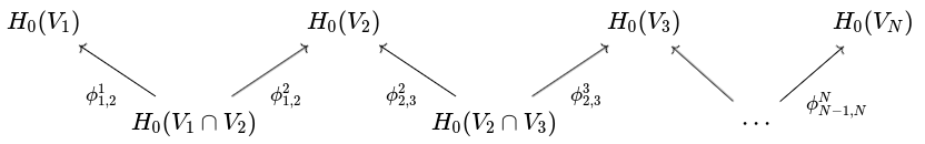
where each ${\varphi }_{i,j}^k:H_0(V_i,V_j)\to H_0(V_k)$, with $k\in \{i,j\}$, is given by inclusion. We can construct the Mapper graph associated to cover $\mathcal{V}$ as follows:

1. For each of the upper spaces, $H_0(V_i)$, we choose the basis $\{v_j^i{\}}_{j=1}^{J_i}$ consisting of the connected components of $V_i$.
2. For each of the lower spaces, $H_0(V_i\cap V_j)$, we choose the basis $\{e_k^{i,i+1}{\}}_{k=1}^{K_i}$. Then the multinerve Mapper graph $\overline{G}$ associated to the zig-zag module is a multigraph defined by vertex sets

$$V(G)=\bigcup _{i=1}^N\{v_1^i,\dots ,v_{J_i}^i\}$$

and edge sets

$$E(G)=\bigcup _{i=1}^{N-1}\left\{{\varphi }_{i,i+1}^i(e_k^{i,i+1}),{\varphi }_{i,i+1}^{i+1}(e_k^{i,i+1}),k=1,\dots ,K_i\right\}.$$

To obtain the Mapper graph $G$, one may take $\overline{G}$ and collapse all parallel edges into single edges.

---

Assuming $f$ is Morse type, this module decomposes into interval modules:

$$EP(f)=\underset{k=1}{\overset{n}{⨁}}\mathbb{I}[b_k,d_k)=\underset{k=1}{\overset{n}{⨁}}\left[(\mathbb{R}\times [b_k,d_k))\cup (\{0\}\times {\mathbb{R}}_{\text{Ext}}-[b_k,d_k))\right].$$

We define a partial matching between persistence diagrams $D$ and $D^{\prime }$ as a subset $\Gamma \subseteq D\times D^{\prime }$ such that if $(p,p^{\prime })\in \Gamma$ and $(p,q^{\prime })\in \Gamma$ then $p^{\prime }=q^{\prime }$ and if $(p,p^{\prime }),(q,p^{\prime })\in \Gamma$ then $p=q$. Let $\Delta \subset {\mathbb{R}}^2$ be the diagonal. Then the cost of $\Gamma$ is defined as

$$\text{cost}(\Gamma ):=\max \left\{\underset{p\in D}{\max }\delta (p),\underset{p^{\prime }\in D^{\prime }}{\max }\delta (p^{\prime })\right\}$$

where $\delta (p)=\Vert p-p^{\prime }{\Vert }_{\infty }$ where $(p,p^{\prime })\in \Gamma$, otherwise $\delta (p)={\inf }_{q\in \Delta }\Vert p-q{\Vert }_{\infty }$. Then the bottleneck distance between $D$ and $D^{\prime }$ is defined by

$$d_b(D,D^{\prime }):=\underset{\Gamma }{\inf }\text{cost}(\Gamma )$$

which ranges over all partial matchings $\Gamma$.